
Time Series Forecasting Lab (Part 2) - Feature Engineering with Recipes

Cover photo by Kristine Tumanyan on Unsplash
Go to R-bloggers for R news and tutorials contributed by hundreds of R bloggers.
This is the second of a series of 6 articles about time series forecasting with panel data and ensemble stacking with R. Click here for Part 1.
Through these articles I will be putting into practice what I have learned from the Business Science University training course 1 DS4B 203-R: High-Performance Time Series Forecasting", delivered by Matt Dancho. If you are looking to gain a high level of expertise in time series with R I strongly recommend this course.
The objective of this article is to explain how to perform time series preprocessing and feature enginneering with timetk . timetk extends recipes for time series.
I will explain what can and cannot be done with recipes for time series panel data.
Introduction
Since the ultimate goal of this series of articles is to perform time series forecast with machine learning, we all know that maximing model performance requires a lot of exprimentation with different feature engineered datasets.
Feature engineering is the most critical part of time series analysis and with recipes you can "use dplyr-like pipeable sequences of feature engineering steps to get your data ready for modeling".
Prerequisites
I assume you are already familiar with the following topics, packages and terms:
time series data format: timestamp, measure, key(s), features
time series lags, rolling lags, Fourier terms
dplyr or tidyverse R packages
normalization and standardization
dummy variables (one-hot encoding)
dataset split into training and test for modeling
Packages
The following packages must be loaded:
# PART 1 - FEATURE ENGINEERING
library(tidyverse)  # loading dplyr, tibble, ggplot2, .. dependencies
library(timetk)  # using timetk plotting, diagnostics and augment operations
library(tsibble)  # for month to Date conversion
library(tsibbledata)  # for aus_retail dataset
library(fastDummies)  # for dummyfying categorical variables
library(skimr) # for quick statistics

# PART 2 -  FEATURE ENGINEERING WITH RECIPES
library(tidymodels)
End-to-end FE process with recipe
Below is a summary diagram of the end-to-end FE process that will be implemented in this article. Notice that the recipe creation will be the last step of the process. The whole process is described hereafter:
Perform measure transformations (here, Turnover) .
Add a future frame with prediction length
Add Fourier, lag, and rolling lag features. Add a rowid column.
Perform a first split into prepared and future datasets.
Apply the training and test split on the prepared dataset.
Create the recipe based upon the training dataset of the split.
Add steps to the recipe such as adding calendar-based features and other tranformations and cleaning.
Recipe limitation for panel data
Generally, we can perform 1., 2., and 3. and preprocessing within a recipe by simply adding the correspong step to it.
The problem is that we are working with panel data , thus it is not possible to include 1., 2., and 3. as different steps within a recipe. We must first perfom these "steps" per group (by "Industry"), and then bind all groups into a single tibble again to be able to do 4., 5., 6. and 7.

Note: the "NA" values in the prepared dataset correspond the (unknown) Turnover predictions within the future frame.
Our data
Let us recall our timeseries dataset from Part 1: the Australian retail trade turnover dataset tsibble::aus_retail filtered by the “Australian Capital Territory” State value."
> aus_retail_tbl <- aus_retail %>%
     tk_tbl()

> monthly_retail_tbl <- aus_retail_tbl %>%
     filter(State == "Australian Capital Territory") %>%
     mutate(Month = as.Date(Month)) %>%
     mutate(Industry = as_factor(Industry)) %>%
     select(Month, Industry, Turnover)

> monthly_retail_tbl %>% glimpse()
Rows: 8,820
Columns: 3
$ Month    <date> 1982-04-01, 1982-05-01, 1982-06-01, 1982-07-01, 1982-08-01, 1982-09-01, 1982-10-01, 1982-11-01, 1982-12-01, 1983-01-01, 1983-02-01, 1983-03-01, 1983-04-01, 1983-05-01,~
$ Industry <fct> "Cafes, restaurants and catering services", "Cafes, restaurants and catering services", "Cafes, restaurants and catering services", "Cafes, restaurants and catering ser~
$ Turnover <dbl> 4.4, 3.4, 3.6, 4.0, 3.6, 4.2, 4.8, 5.4, 6.9, 3.8, 4.2, 4.0, 4.4, 4.3, 4.3, 4.6, 4.9, 4.5, 5.5, 6.7, 9.6, 3.8, 3.8, 4.4, 3.8, 3.9, 4.1, 4.3, 4.8, 5.0, 5.3, 5.6, 6.8, 4.6~
The code snippet below will steps (not recipe steps!) 1., 2., and 3. as explained above. You can always refer to Part 1 for function arguments explanations.
We will generate a list (groups) of 20 tibbles, each corresponding to a specific industry. In addition to steps 1., 2. and 3. I have also arranged in ascending order the timestamp (Month) for each Industry group for the lags, rolling lags and Fourier terms.
We add a future frame, starting from 2019-01-01 to 2019-12-01 (12-month length), which will hold NA values for the measure (Turnover) but to which the Fourier, lag and rolling lag features will also be added.
Finally, we bind them together to produce the first feature engineered tibble groups_fe_tbl.
groups <- lapply(X = 1:length(Industries), FUN = function(x){

  monthly_retail_tbl %>%
    filter(Industry == Industries[x]) %>%
    arrange(Month) %>%
    mutate(Turnover =  log1p(x = Turnover)) %>%
    mutate(Turnover =  standardize_vec(Turnover)) %>%
    future_frame(Month, .length_out = "12 months", .bind_data = TRUE) %>%
    mutate(Industry = Industries[x]) %>%
    tk_augment_fourier(.date_var = Month, .periods = 12, .K = 1) %>%
    tk_augment_lags(.value = Turnover, .lags = 12) %>%
    tk_augment_slidify(.value   = Turnover_lag12,
                       .f       = ~ mean(.x, na.rm = TRUE),
                       .period  = c(3, 6, 9, 12),
                       .partial = TRUE,
                       .align   = "center")
})

groups_fe_tbl <- bind_rows(groups) %>%
  rowid_to_column(var = "rowid")
Below I will display the last 13 months of groups_fe_tbl, you should see the last historical row (2018-12-01) and the future frame values for the last industry (obviously, we have the same situation for other industries within the same tibble):
> groups_fe_tbl %>% tail(n=13) %>% glimpse()
Rows: 13
Columns: 16
$ rowid                  <int> 9048, 9049, 9050, 9051, 9052, 9053, 9054, 9055, 9056, 9057, 9058, 9059, 9060
$ Month                  <date> 2018-12-01, 2019-01-01, 2019-02-01, 2019-03-01, 2019-04-01, 2019-05-01, 2019-06-01, 2019-07-01, 20~
$ Industry               <chr> "Takeaway food services", "Takeaway food services", "Takeaway food services", "Takeaway food serv~
$ Turnover               <dbl> 2.078015, NA, NA, NA, NA, NA, NA, NA, NA, NA, NA, NA, NA
$ Month_sin12_K1         <dbl> 0.16810089, 0.63846454, 0.93775213, 0.99301874, 0.80100109, 0.40982032, -0.10116832, -0.57126822, ~
$ Month_cos12_K1         <dbl> 0.98576980, 0.76965124, 0.34730525, -0.11795672, -0.59866288, -0.91216627, -0.99486932, -0.8207634~
$ Turnover_lag12         <dbl> 1.668977, 1.397316, 1.542003, 1.894938, 1.894938, 1.894938, 1.878972, 1.886969, 1.957669, 1.926527~
$ Turnover_lag13         <dbl> 1.755391, 1.668977, 1.397316, 1.542003, 1.894938, 1.894938, 1.894938, 1.878972, 1.886969, 1.957669~
$ Turnover_lag12_roll_3  <dbl> 1.607228, 1.536098, 1.611419, 1.777293, 1.894938, 1.889616, 1.886960, 1.907870, 1.923722, 1.972616~
$ Turnover_lag13_roll_3  <dbl> 1.723756, 1.607228, 1.536098, 1.611419, 1.777293, 1.894938, 1.889616, 1.886960, 1.907870, 1.923722~
$ Turnover_lag12_roll_6  <dbl> 1.667587, 1.692260, 1.715518, 1.750517, 1.832126, 1.901404, 1.906669, 1.929788, 1.941529, 1.974703~
$ Turnover_lag13_roll_6  <dbl> 1.668911, 1.667587, 1.692260, 1.715518, 1.750517, 1.832126, 1.901404, 1.906669, 1.929788, 1.941529~
$ Turnover_lag12_roll_9  <dbl> 1.750363, 1.744253, 1.741597, 1.757160, 1.779636, 1.808252, 1.878956, 1.925999, 1.946341, 1.952766~
$ Turnover_lag13_roll_9  <dbl> 1.748589, 1.750363, 1.744253, 1.741597, 1.757160, 1.779636, 1.808252, 1.878956, 1.925999, 1.929881~
$ Turnover_lag12_roll_12 <dbl> 1.783846, 1.784512, 1.785157, 1.787128, 1.811024, 1.828524, 1.862610, 1.904910, 1.941200, 1.946341~
$ Turnover_lag13_roll_12 <dbl> 1.766346, 1.783846, 1.784512, 1.785157, 1.787128, 1.811024, 1.828524, 1.843028, 1.887599, 1.925999~
Save standarization parameters
Since we are working with panel data (there are 20 time series, one for each Industry), consequently there will be 20 Standardization Parameters (mean, standard deviation) generated by standardize_vec(Turnover).
The values of these parameters must be saved, Ajay Mehta proposed an elegant solution with group_map(), I'm including his code snippet based on his comment at the end of this article. The mean and standard deviation values will be saved in std_mean and std_sd vectors respectively.
tmp <- monthly_retail_tbl %>%
  group_by(Industry) %>%
  arrange(Month) %>%
  mutate(Turnover = log1p(x = Turnover)) %>%
  group_map(~ c(mean = mean(.x$Turnover, na.rm = TRUE),
                sd = sd(.x$Turnover, na.rm = TRUE))) %>%
  bind_rows()

std_mean <- tmp$mean
std_sd <- tmp$sd
rm('tmp')
Prepared and future datasets
We perform the split of groups_fe_tbl into prepared and future datasets .
The prepared dataset is the one with historic values of the measure (here Turnover) which must not have NA values. Although we know Turnover does have missing values we still apply filter(!is.na(Turnover)). We will also drop all rows with NA values elsewhere e.g., those introduced by lag and rolling lag features.
Finally, we obtain an 8,560-row tibble (data_prepared_tbl ) from a 9,060-row one (groups_fe_tbl). You can run a groups_fe_tbl %>% group_by(Industry) %>% skim() to check the total number of missing values (NA and NaN ) that were removed.
Prepared dataset starts from 1983-04-01.
> data_prepared_tbl <- groups_fe_tbl %>%
    filter(!is.na(Turnover)) %>%
    drop_na()

> data_prepared_tbl %>% glimpse()
Rows: 8,560
Columns: 16
$ rowid                  <int> 14, 15, 16, 17, 18, 19, 20, 21, 22, 23, 24, 25, 26, 27, 28, 29, 30, 31, 32, 33, 34, 35, 36, 37, 38~
$ Month                  <date> 1983-05-01, 1983-06-01, 1983-07-01, 1983-08-01, 1983-09-01, 1983-10-01, 1983-11-01, 1983-12-01, 1~
$ Industry               <chr> "Cafes, restaurants and catering services", "Cafes, restaurants and catering services", "Cafes, re~
$ Turnover               <dbl> -2.0426107, -2.0426107, -1.9499231, -1.8620736, -1.9802554, -1.6990366, -1.4138382, -0.8757670, -2~
$ Month_sin12_K1         <dbl> 0.51455540, 0.87434662, 1.00000000, 0.86602540, 0.50000000, 0.01688948, -0.48530196, -0.84864426, ~
$ Month_cos12_K1         <dbl> 8.574571e-01, 4.853020e-01, 1.567970e-14, -5.000000e-01, -8.660254e-01, -9.998574e-01, -8.743466e-~
$ Turnover_lag12         <dbl> -2.355895, -2.281065, -2.140701, -2.281065, -2.074676, -1.890850, -1.725136, -1.370672, -2.209420,~
$ Turnover_lag13         <dbl> -2.011144, -2.355895, -2.281065, -2.140701, -2.281065, -2.074676, -1.890850, -1.725136, -1.370672,~
$ Turnover_lag12_roll_3  <dbl> -2.216035, -2.259220, -2.234277, -2.165481, -2.082197, -1.896888, -1.662219, -1.768409, -1.884923,~
$ Turnover_lag13_roll_3  <dbl> -2.183520, -2.216035, -2.259220, -2.234277, -2.165481, -2.082197, -1.896888, -1.662219, -1.768409,~
$ Turnover_lag12_roll_6  <dbl> -2.213974, -2.190758, -2.170709, -2.065582, -1.913850, -1.925303, -1.890905, -1.901909, -1.921958,~
$ Turnover_lag13_roll_6  <dbl> -2.197201, -2.213974, -2.190758, -2.170709, -2.065582, -1.913850, -1.925303, -1.890905, -1.901909,~
$ Turnover_lag12_roll_9  <dbl> -2.190758, -2.147914, -2.095067, -2.014578, -2.036609, -2.005362, -1.989766, -1.975371, -1.948876,~
$ Turnover_lag13_roll_9  <dbl> -2.213974, -2.190758, -2.147914, -2.095067, -2.014578, -2.036609, -2.005362, -1.989766, -1.975371,~
$ Turnover_lag12_roll_12 <dbl> -2.095067, -2.014578, -2.034063, -2.037755, -2.046334, -2.046334, -2.020226, -2.000355, -1.984457,~
$ Turnover_lag13_roll_12 <dbl> -2.147914, -2.095067, -2.014578, -2.034063, -2.037755, -2.046334, -2.046334, -2.020226, -2.000355,~
The future dataset hold the 12 future (and unknown) values of Turnover e.g., the NA values introduced by the future frame. We will predict and fill in the values in Part 6 with the final stacking ensemble model.
> future_tbl <- groups_fe_tbl %>%
    filter(is.na(Turnover))

> future_tbl %>% head(n=12) %>% glimpse()
Rows: 12
Columns: 16
$ rowid                  <int> 442, 443, 444, 445, 446, 447, 448, 449, 450, 451, 452, 453
$ Month                  <date> 2019-01-01, 2019-02-01, 2019-03-01, 2019-04-01, 2019-05-01, 2019-06-01, 2019-07-01, 2019-08-01, 20~
$ Industry               <chr> "Cafes, restaurants and catering services", "Cafes, restaurants and catering services", "Cafes, r~
$ Turnover               <dbl> NA, NA, NA, NA, NA, NA, NA, NA, NA, NA, NA, NA
$ Month_sin12_K1         <dbl> 0.63846454, 0.93775213, 0.99301874, 0.80100109, 0.40982032, -0.10116832, -0.57126822, -0.90511451,~
$ Month_cos12_K1         <dbl> 0.76965124, 0.34730525, -0.11795672, -0.59866288, -0.91216627, -0.99486932, -0.82076344, -0.425167~
$ Turnover_lag12         <dbl> 1.125397, 1.282320, 1.569292, 1.425855, 1.437951, 1.429897, 1.550608, 1.469789, 1.457920, 1.469789~
$ Turnover_lag13         <dbl> 1.384894, 1.125397, 1.282320, 1.569292, 1.425855, 1.437951, 1.429897, 1.550608, 1.469789, 1.457920~
$ Turnover_lag12_roll_3  <dbl> 1.264204, 1.325670, 1.425822, 1.477699, 1.431234, 1.472819, 1.483431, 1.492773, 1.465833, 1.495272~
$ Turnover_lag13_roll_3  <dbl> 1.316081, 1.264204, 1.325670, 1.425822, 1.477699, 1.431234, 1.472819, 1.483431, 1.492773, 1.465833~
$ Turnover_lag12_roll_6  <dbl> 1.370952, 1.370952, 1.378452, 1.449320, 1.480565, 1.462003, 1.469326, 1.489352, 1.490694, 1.478711~
$ Turnover_lag13_roll_6  <dbl> 1.378274, 1.370952, 1.370952, 1.378452, 1.449320, 1.480565, 1.462003, 1.469326, 1.489352, 1.501243~
$ Turnover_lag12_roll_9  <dbl> 1.411416, 1.395927, 1.404907, 1.408445, 1.416559, 1.454825, 1.485468, 1.470874, 1.476502, 1.482009~
$ Turnover_lag13_roll_9  <dbl> 1.420563, 1.411416, 1.395927, 1.404907, 1.408445, 1.416559, 1.454825, 1.485468, 1.474990, 1.482009~
$ Turnover_lag12_roll_12 <dbl> 1.433627, 1.429420, 1.420139, 1.420139, 1.430152, 1.434573, 1.462680, 1.480716, 1.470874, 1.476502~
$ Turnover_lag13_roll_12 <dbl> 1.429496, 1.433627, 1.429420, 1.420139, 1.420139, 1.430152, 1.434266, 1.465153, 1.485468, 1.474990~
Train and test datasets split
We perform the split with timetk::time_series_split() function. The latter returns a split object (an R list) which can be further used for plotting both the traininig and the test datasets.
One important argument is assess, it determines the length of the test dataset. As per 2 , "The size of the test set is typically about 20% of the total sample, although this value depends on how long the sample is and how far ahead you want to forecast. The test dataset should ideally be at least as large as the maximum forecast horizon required." Since there are 428 observations (months) per industry, then 20% of 428 is 86 months (rounded up).
cumulative = TRUE means that we consider the training dataset from the begining (first row) of the prepared dataset.
> splits <- data_prepared_tbl %>%
    time_series_split(Month,
                      assess = "86 months",
                      cumulative = TRUE)

# split object
> splits
<Analysis/Assess/Total>
<6840/1720/8560>
Which means
6840 rows for training (all 20 industries). Here, we only care about the rows since the number of columns will be updated by the recipe (explained soon).
1720 rows for test dataset (86 months x 20 industries)
8560 rows of
data_prepared_tbl(all 20 industries)
You can confirm the size of the training and test datasets with the following code snippet using the tk_time_series_cv_plan() function which creates a new tibble with two new columns .id and .key
> splits %>%
   tk_time_series_cv_plan() %>% glimpse()
Rows: 8,560
Columns: 18
$ .id                    <chr> "Slice1", "Slice1", "Slice1", "Slice1", "Slice1", "Slice1", "Slice1", "Slice1", "Slice1", "Slic~
$ .key                   <fct> training, training, training, training, training, training, training, training, training, train~
$ rowid                  <int> 14, 467, 920, 1373, 1826, 2279, 2732, 3185, 3638, 4091, 4544, 4997, 5450, 5903, 6356, 6809, 726~
$ Month                  <date> 1983-05-01, 1983-05-01, 1983-05-01, 1983-05-01, 1983-05-01, 1983-05-01, 1983-05-01, 1983-05-01~
$ Industry               <chr> "Cafes, restaurants and catering services", "Cafes, restaurants and takeaway food services", "C~
$ Turnover               <dbl> -2.042611, -1.866127, -1.383977, -1.533674, -1.772910, -1.575604, -1.941481, -1.635071, -1.9995~
$ Month_sin12_K1         <dbl> 0.5145554, 0.5145554, 0.5145554, 0.5145554, 0.5145554, 0.5145554, 0.5145554, 0.5145554, 0.51455~
$ Month_cos12_K1         <dbl> 8.574571e-01, 8.574571e-01, 8.574571e-01, 8.574571e-01, 8.574571e-01, 8.574571e-01, 8.574571e-0~
$ Turnover_lag12         <dbl> -2.355895, -2.397538, -1.674143, -1.891997, -1.973832, -1.550576, -2.113506, -2.109525, -2.2924~
$ Turnover_lag13         <dbl> -2.011144, -2.195619, -1.713772, -1.891997, -2.044287, -1.680229, -2.080545, -2.035540, -2.4340~
$ Turnover_lag12_roll_3  <dbl> -2.216035, -2.299396, -1.771137, -1.971674, -2.053104, -1.602136, -2.091532, -2.110334, -2.4204~
$ Turnover_lag13_roll_3  <dbl> -2.183520, -2.296579, -1.693957, -1.891997, -2.009059, -1.615402, -2.097026, -2.072532, -2.3632~
$ Turnover_lag12_roll_6  <dbl> -2.213974, -2.275130, -1.824439, -2.023204, -2.202758, -1.587032, -2.072703, -2.125292, -2.4065~
$ Turnover_lag13_roll_6  <dbl> -2.197201, -2.278793, -1.787835, -1.988232, -2.146638, -1.577044, -2.076792, -2.110131, -2.4117~
$ Turnover_lag12_roll_9  <dbl> -2.190758, -2.244673, -1.826687, -2.015706, -2.222243, -1.607126, -2.067327, -2.110334, -2.4193~
$ Turnover_lag13_roll_9  <dbl> -2.213974, -2.275130, -1.824439, -2.023204, -2.202758, -1.587032, -2.072703, -2.125292, -2.4065~
$ Turnover_lag12_roll_12 <dbl> -2.095067, -2.152525, -1.819038, -1.978000, -2.167591, -1.593199, -2.043333, -2.048362, -2.3049~
$ Turnover_lag13_roll_12 <dbl> -2.147914, -2.200931, -1.828293, -2.002079, -2.217778, -1.606260, -2.056832, -2.089405, -2.3594~

> splits %>%
   tk_time_series_cv_plan() %>% select(.id) %>% table()

Slice1
  8560

> splits %>%
   tk_time_series_cv_plan() %>% select(.key) %>% table()

training  testing
    6840     1720
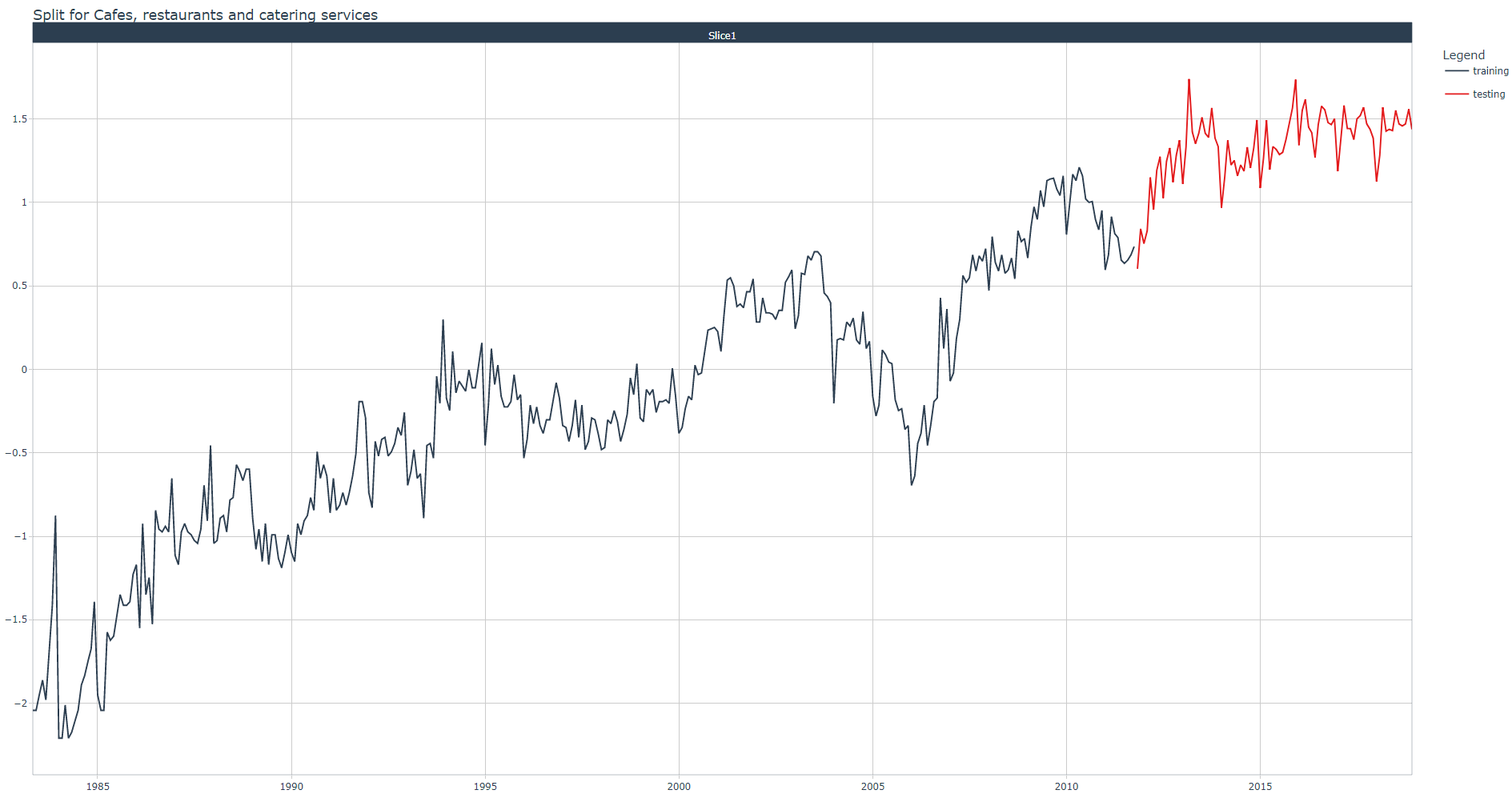
Let us plot the training and test datasets for one Industry value with the plot_time_series_cv_plan() function:
> Industries <- unique(aus_retail_tbl$Industry)
> splits %>%
  tk_time_series_cv_plan() %>%
  filter(Industry == Industries[1]) %>%
  plot_time_series_cv_plan(.date_var = Month,
                           .value = Turnover,
                           .title = paste0("Split for ", industry))
You can extract the training and test datasets by applying the training() and testing() functions respectively on the splits object.
> training(splits) %>%
     filter(Industry == Industries[industry]) %>%
     glimpse()
Rows: 342
Columns: 16
$ rowid                  <int> 14, 15, 16, 17, 18, 19, 20, 21, 22, 23, 24, 25, 26, 27, 28, 29, 30, 31, 32, 33, 34, 35, 36, 37,~
$ Month                  <date> 1983-05-01, 1983-06-01, 1983-07-01, 1983-08-01, 1983-09-01, 1983-10-01, 1983-11-01, 1983-12-01~
$ Industry               <chr> "Cafes, restaurants and catering services", "Cafes, restaurants and catering services", "Cafes,~
$ Turnover               <dbl> -2.0426107, -2.0426107, -1.9499231, -1.8620736, -1.9802554, -1.6990366, -1.4138382, -0.8757670,~
$ Month_sin12_K1         <dbl> 0.51455540, 0.87434662, 1.00000000, 0.86602540, 0.50000000, 0.01688948, -0.48530196, -0.8486442~
$ Month_cos12_K1         <dbl> 8.574571e-01, 4.853020e-01, 1.567970e-14, -5.000000e-01, -8.660254e-01, -9.998574e-01, -8.74346~
$ Turnover_lag12         <dbl> -2.355895, -2.281065, -2.140701, -2.281065, -2.074676, -1.890850, -1.725136, -1.370672, -2.2094~
$ Turnover_lag13         <dbl> -2.011144, -2.355895, -2.281065, -2.140701, -2.281065, -2.074676, -1.890850, -1.725136, -1.3706~
$ Turnover_lag12_roll_3  <dbl> -2.216035, -2.259220, -2.234277, -2.165481, -2.082197, -1.896888, -1.662219, -1.768409, -1.8849~
$ Turnover_lag13_roll_3  <dbl> -2.183520, -2.216035, -2.259220, -2.234277, -2.165481, -2.082197, -1.896888, -1.662219, -1.7684~
$ Turnover_lag12_roll_6  <dbl> -2.213974, -2.190758, -2.170709, -2.065582, -1.913850, -1.925303, -1.890905, -1.901909, -1.9219~
$ Turnover_lag13_roll_6  <dbl> -2.197201, -2.213974, -2.190758, -2.170709, -2.065582, -1.913850, -1.925303, -1.890905, -1.9019~
$ Turnover_lag12_roll_9  <dbl> -2.190758, -2.147914, -2.095067, -2.014578, -2.036609, -2.005362, -1.989766, -1.975371, -1.9488~
$ Turnover_lag13_roll_9  <dbl> -2.213974, -2.190758, -2.147914, -2.095067, -2.014578, -2.036609, -2.005362, -1.989766, -1.9753~
$ Turnover_lag12_roll_12 <dbl> -2.095067, -2.014578, -2.034063, -2.037755, -2.046334, -2.046334, -2.020226, -2.000355, -1.9844~
$ Turnover_lag13_roll_12 <dbl> -2.147914, -2.095067, -2.014578, -2.034063, -2.037755, -2.046334, -2.046334, -2.020226, -2.0003~
It is important to understand that the actual training dataset to be used to learn the model will be the output of the recipe , as explained hereafter.
Create recipe
As stated in Get Started, before training the model, we can use a recipe to create (new) predictors and conduct the preprocessing required by the model.
recipe(Turnover ~ ., data = training(splits))
"The recipe() function as we used it here has two arguments:
A formula. Any variable on the left-hand side of the tilde (~) is considered the model outcome (here,
Turnover). On the right-hand side of the tilde are the predictors. Variables may be listed by name, or you can use the dot (.) to indicate all other variables as predictors.The data. A recipe is associated with the data set used to create the model. This will typically be the training set, so data =
training(splits)here. Naming a data set doesn’t actually change the data itself; it is only used to catalog the names of the variables and their types, like factors, integers, dates, etc."
For each preprocessing and feature engineering steps explained in Part 1 there is a specific step_<> :
add calendar-based features:
step_timeseries_signature()remove columns:
step_rm()perform one-hot encoding on categorical variables:
step_dummy()normalize numeric variables:
step_normalize()
recipe_spec <- recipe(Turnover ~ ., data = training(splits)) %>%
  update_role(rowid, new_role = "indicator") %>%
  step_other(Industry) %>%
  step_timeseries_signature(Month) %>%
  step_rm(matches("(.xts$)|(.iso$)|(hour)|(minute)|(second)|(day)|(week)|(am.pm)")) %>%
  step_dummy(all_nominal(), one_hot = TRUE) %>%
  step_normalize(Month_index.num, Month_year)
Notice the two very useful functions explained hereafter:
update_role(rowid, new_role = "indicator"): it lets recipes know that rowid variable has a custom role called "indicator" (a role can have any character value). This tells the recipe to keep the rowid variable without using it neither as an outcome nor a predictor.
step_other(Industry): in case the training dataset does not include all Industry (categorical variable) values, it will pool the infrequently occurring values into an "other" category.
Below we display the recipe's spec, its summary, and finally the (real) training dataset:
> recipe_spec
Recipe

Inputs:

      role #variables
 indicator          1
   outcome          1
 predictor         14

Operations:

Collapsing factor levels for Industry
Timeseries signature features from Month
Delete terms matches("(.xts$)|(.iso$)|(hour)|(minute)|(second)|(day)|(week)|(am.pm)")
Dummy variables from all_nominal()
Centering and scaling for Month_index.num, Month_year

# Recipe summary: 50 predictors (including all dummy variables) + 1 indicator + 1 outcome
> recipe_spec %>%
+   prep() %>%
+   summary()
# A tibble: 52 x 4
   variable              type    role      source
   <chr>                 <chr>   <chr>     <chr>
 1 rowid                 numeric indicator original
 2 Month                 date    predictor original
 3 Month_sin12_K1        numeric predictor original
 4 Month_cos12_K1        numeric predictor original
 5 Turnover_lag12        numeric predictor original
 6 Turnover_lag13        numeric predictor original
 7 Turnover_lag12_roll_3 numeric predictor original
 8 Turnover_lag13_roll_3 numeric predictor original
 9 Turnover_lag12_roll_6 numeric predictor original
10 Turnover_lag13_roll_6 numeric predictor original
# ... with 42 more rows

# Extracted training dataset
> recipe_spec %>%
   prep() %>%
   juice() %>%
   glimpse()
Rows: 6,840
Columns: 52
$ rowid                                                                      <int> 14, 467, 920, 1373, 1826, 2279, 2732, 3185,~
$ Month                                                                      <date> 1983-05-01, 1983-05-01, 1983-05-01, 1983-0~
$ Month_sin12_K1                                                             <dbl> 0.5145554, 0.5145554, 0.5145554, 0.5145554,~
$ Month_cos12_K1                                                             <dbl> 8.574571e-01, 8.574571e-01, 8.574571e-01, 8~
$ Turnover_lag12                                                             <dbl> -2.355895, -2.397538, -1.674143, -1.891997,~
$ Turnover_lag13                                                             <dbl> -2.011144, -2.195619, -1.713772, -1.891997,~
$ Turnover_lag12_roll_3                                                      <dbl> -2.216035, -2.299396, -1.771137, -1.971674,~
$ Turnover_lag13_roll_3                                                      <dbl> -2.183520, -2.296579, -1.693957, -1.891997,~
$ Turnover_lag12_roll_6                                                      <dbl> -2.213974, -2.275130, -1.824439, -2.023204,~
$ Turnover_lag13_roll_6                                                      <dbl> -2.197201, -2.278793, -1.787835, -1.988232,~
$ Turnover_lag12_roll_9                                                      <dbl> -2.190758, -2.244673, -1.826687, -2.015706,~
$ Turnover_lag13_roll_9                                                      <dbl> -2.213974, -2.275130, -1.824439, -2.023204,~
$ Turnover_lag12_roll_12                                                     <dbl> -2.095067, -2.152525, -1.819038, -1.978000,~
$ Turnover_lag13_roll_12                                                     <dbl> -2.147914, -2.200931, -1.828293, -2.002079,~
$ Turnover                                                                   <dbl> -2.042611, -1.866127, -1.383977, -1.533674,~
$ Month_index.num                                                            <dbl> -1.727262, -1.727262, -1.727262, -1.727262,~
$ Month_year                                                                 <dbl> -1.710287, -1.710287, -1.710287, -1.710287,~
$ Month_half                                                                 <int> 1, 1, 1, 1, 1, 1, 1, 1, 1, 1, 1, 1, 1, 1, 1~
$ Month_quarter                                                              <int> 2, 2, 2, 2, 2, 2, 2, 2, 2, 2, 2, 2, 2, 2, 2~
$ Month_month                                                                <int> 5, 5, 5, 5, 5, 5, 5, 5, 5, 5, 5, 5, 5, 5, 5~
$ Industry_Cafes..restaurants.and.catering.services                          <dbl> 1, 0, 0, 0, 0, 0, 0, 0, 0, 0, 0, 0, 0, 0, 0~
$ Industry_Cafes..restaurants.and.takeaway.food.services                     <dbl> 0, 1, 0, 0, 0, 0, 0, 0, 0, 0, 0, 0, 0, 0, 0~
$ Industry_Clothing.retailing                                                <dbl> 0, 0, 1, 0, 0, 0, 0, 0, 0, 0, 0, 0, 0, 0, 0~
$ Industry_Clothing..footwear.and.personal.accessory.retailing               <dbl> 0, 0, 0, 1, 0, 0, 0, 0, 0, 0, 0, 0, 0, 0, 0~
$ Industry_Department.stores                                                 <dbl> 0, 0, 0, 0, 1, 0, 0, 0, 0, 0, 0, 0, 0, 0, 0~
$ Industry_Electrical.and.electronic.goods.retailing                         <dbl> 0, 0, 0, 0, 0, 1, 0, 0, 0, 0, 0, 0, 0, 0, 0~
$ Industry_Food.retailing                                                    <dbl> 0, 0, 0, 0, 0, 0, 1, 0, 0, 0, 0, 0, 0, 0, 0~
$ Industry_Footwear.and.other.personal.accessory.retailing                   <dbl> 0, 0, 0, 0, 0, 0, 0, 1, 0, 0, 0, 0, 0, 0, 0~
$ Industry_Furniture..floor.coverings..houseware.and.textile.goods.retailing <dbl> 0, 0, 0, 0, 0, 0, 0, 0, 1, 0, 0, 0, 0, 0, 0~
$ Industry_Hardware..building.and.garden.supplies.retailing                  <dbl> 0, 0, 0, 0, 0, 0, 0, 0, 0, 1, 0, 0, 0, 0, 0~
$ Industry_Household.goods.retailing                                         <dbl> 0, 0, 0, 0, 0, 0, 0, 0, 0, 0, 1, 0, 0, 0, 0~
$ Industry_Liquor.retailing                                                  <dbl> 0, 0, 0, 0, 0, 0, 0, 0, 0, 0, 0, 1, 0, 0, 0~
$ Industry_Newspaper.and.book.retailing                                      <dbl> 0, 0, 0, 0, 0, 0, 0, 0, 0, 0, 0, 0, 1, 0, 0~
$ Industry_Other.recreational.goods.retailing                                <dbl> 0, 0, 0, 0, 0, 0, 0, 0, 0, 0, 0, 0, 0, 1, 0~
$ Industry_Other.retailing                                                   <dbl> 0, 0, 0, 0, 0, 0, 0, 0, 0, 0, 0, 0, 0, 0, 1~
$ Industry_Other.retailing.n.e.c.                                            <dbl> 0, 0, 0, 0, 0, 0, 0, 0, 0, 0, 0, 0, 0, 0, 0~
$ Industry_Other.specialised.food.retailing                                  <dbl> 0, 0, 0, 0, 0, 0, 0, 0, 0, 0, 0, 0, 0, 0, 0~
$ Industry_Pharmaceutical..cosmetic.and.toiletry.goods.retailing             <dbl> 0, 0, 0, 0, 0, 0, 0, 0, 0, 0, 0, 0, 0, 0, 0~
$ Industry_Supermarket.and.grocery.stores                                    <dbl> 0, 0, 0, 0, 0, 0, 0, 0, 0, 0, 0, 0, 0, 0, 0~
$ Industry_Takeaway.food.services                                            <dbl> 0, 0, 0, 0, 0, 0, 0, 0, 0, 0, 0, 0, 0, 0, 0~
$ Month_month.lbl_01                                                         <dbl> 0, 0, 0, 0, 0, 0, 0, 0, 0, 0, 0, 0, 0, 0, 0~
$ Month_month.lbl_02                                                         <dbl> 0, 0, 0, 0, 0, 0, 0, 0, 0, 0, 0, 0, 0, 0, 0~
$ Month_month.lbl_03                                                         <dbl> 0, 0, 0, 0, 0, 0, 0, 0, 0, 0, 0, 0, 0, 0, 0~
$ Month_month.lbl_04                                                         <dbl> 0, 0, 0, 0, 0, 0, 0, 0, 0, 0, 0, 0, 0, 0, 0~
$ Month_month.lbl_05                                                         <dbl> 1, 1, 1, 1, 1, 1, 1, 1, 1, 1, 1, 1, 1, 1, 1~
$ Month_month.lbl_06                                                         <dbl> 0, 0, 0, 0, 0, 0, 0, 0, 0, 0, 0, 0, 0, 0, 0~
$ Month_month.lbl_07                                                         <dbl> 0, 0, 0, 0, 0, 0, 0, 0, 0, 0, 0, 0, 0, 0, 0~
$ Month_month.lbl_08                                                         <dbl> 0, 0, 0, 0, 0, 0, 0, 0, 0, 0, 0, 0, 0, 0, 0~
$ Month_month.lbl_09                                                         <dbl> 0, 0, 0, 0, 0, 0, 0, 0, 0, 0, 0, 0, 0, 0, 0~
$ Month_month.lbl_10                                                         <dbl> 0, 0, 0, 0, 0, 0, 0, 0, 0, 0, 0, 0, 0, 0, 0~
$ Month_month.lbl_11                                                         <dbl> 0, 0, 0, 0, 0, 0, 0, 0, 0, 0, 0, 0, 0, 0, 0~
$ Month_month.lbl_12                                                         <dbl> 0, 0, 0, 0, 0, 0, 0, 0, 0, 0, 0, 0, 0, 0, 0~
As for the standardization parameters, we save the normalization parameters generated by the step_normalize() function applied on Month_index.num and Month_year columns. Min-max normalization was used for these columns.
To get the original min and max values prior normalization you must customize the skim() function as I did in Part 1 with my myskim() functionand apply it to training(splits).
recipe(Turnover ~ ., data = training(splits)) %>%
  step_timeseries_signature(Month) %>%
  prep() %>%
  juice() %>%
  myskim()

# Extract of the output for the sake of clarity:
... ...

-- Variable type: numeric ------------------------------------------------------------------------------------------------------------------------------------------------------------------------
   skim_variable          n_missing complete_rate     mean            sd           p0           p25      p50     p75          p100           max          min

 ... ...

15 Month_index.num                0             1  8.69e+8 259648888.    420595200    644198400      8.69e+8 1.09e+9 1317427200    1317427200    420595200
16 Month_year                     0             1  2.00e+3         8.23       1983         1990      2.00e+3 2.00e+3       2011          2011         1983

... ...

# Month_index.num normalization Parameters
Month_index.num_limit_lower = 420595200
Month_index.num_limit_upper = 1317427200

# Month_year normalization Parameters
Month_year_limit_lower = 1983
Month_year_limit_upper = 2011
Save your work
We will keep all data, recipes, splits, parameters and any other useful stuff in a list and save it as an RDS file.
feature_engineering_artifacts_list <- list(
  # Data
  data = list(
    data_prepared_tbl = data_prepared_tbl,
    future_tbl      = future_tbl,
    industries = Industries
  ),

  # Recipes
  recipes = list(
    recipe_spec = recipe_spec
  ),

  # Splits
  splits = splits,

  # Inversion Parameters
  standardize = list(
    std_mean = std_mean,
    std_sd   = std_sd
  ),

  normalize = list(
    Month_index.num_limit_lower = Month_index.num_limit_lower,
    Month_index.num_limit_upper = Month_index.num_limit_upper,
    Month_year_limit_lower = Month_year_limit_lower,
    Month_year_limit_upper = Month_year_limit_upper
  )
)

feature_engineering_artifacts_list %>%
  write_rds("feature_engineering_artifacts_list.rds")
Conclusion
In this article I have explained how to perform time series feature engineering with recipes thanks to the timetk package.
The recipe performed preprocessing, transformations and feature engineering applicable to all 20 time series (panel data). For operations such as measure standardization, adding lags, rolling lags and Fourier terms we needed to code a specific by group (here, by Industry) feature engineering.
The recipe is an important step in the data science process with modeltime since it will be added to a workflow along with a model, this will be explained in my next article (Part 3).
Note: I haven't shown all the power of recipes e.g., model-specific recipes can be built from a "base" recipe which can be modified in order to adapt to the model requirements. Remember, it is important to perform experimentation with different datasets and creating interdependent recipes can be very useful.
References
1 Dancho, Matt, "DS4B 203-R: High-Performance Time Series Forecasting", Business Science University
2 Hyndman R., Athanasopoulos G., "Forecasting: Principles and Practice", 3rd edition