
Time Series Forecasting Lab (Part 1) - Introduction to Feature Engineering

Cover photo by Mourizal Zativa on Unsplash
Go to R-bloggers for R news and tutorials contributed by hundreds of R bloggers.
Introduction
This is the first of a series of 6 articles about time series forecasting with panel data and ensemble stacking with R.
Through these articles I will be putting into practice what I have learned from the Business Science University training course 2 DS4B 203-R: High-Performance Time Series Forecasting", delivered by Matt Dancho. If you are looking to gain a high level of expertise in time series with R I strongly recommend this course.
The objective of this article is to show how easy it is to perform time series feature engineering with the timetk package, by adding some common and very useful features to a time series dataset. Step by step, we will be adding calendar-based features, Fourier terms, lag and rolling lag features.

Prerequisites
I assume you are already familiar with the following topics, packages and terms:
- time series data format: timestamp, measure, key(s), features
- time series lags, rolling lags, Fourier terms
- dplyr or tidyverse R packages
- normalization and standardization
- dummy variables (one-hot encoding)
- linear regression
- adjusted R-squared
Packages
The following packages must be loaded:
# PART 1 -  FEATURE ENGINEERING
library(tidyverse)  # loading dplyr, tibble, ggplot2, .. dependencies
library(timetk)  # using timetk plotting, diagnostics and augment operations
library(tsibble)  # for month to Date conversion
library(tsibbledata)  # for aus_retail dataset
library(fastDummies)  # for dummyfying categorical variables
library(skimr) # for quick statistics
Data
Let us load the Australian retail trade turnover dataset tsibble::aus_retail
. The time series measure is Turnover which represents the retail turnover in $Million AUD.
Our final goal is to forecast Turnover for the next year.
Within the dataset each series is uniquely identified using two keys:
- State: The Australian state (or territory)
- Industry: The industry of retail trade
We will focus on the “Australian Capital Territory” State value only and use all Industry values.
> tsibbledata::aus_retail
# A tsibble: 64,532 x 5 [1M]
# Key:       State, Industry [152]
   State                        Industry                                 `Series ID`    Month Turnover
   <chr>                        <chr>                                    <chr>          <mth>    <dbl>
 1 Australian Capital Territory Cafes, restaurants and catering services A3349849A   1982 Apr      4.4
 2 Australian Capital Territory Cafes, restaurants and catering services A3349849A   1982 May      3.4
 3 Australian Capital Territory Cafes, restaurants and catering services A3349849A   1982 Jun      3.6
 4 Australian Capital Territory Cafes, restaurants and catering services A3349849A   1982 Jul      4
 5 Australian Capital Territory Cafes, restaurants and catering services A3349849A   1982 Aug      3.6
 6 Australian Capital Territory Cafes, restaurants and catering services A3349849A   1982 Sep      4.2
 7 Australian Capital Territory Cafes, restaurants and catering services A3349849A   1982 Oct      4.8
 8 Australian Capital Territory Cafes, restaurants and catering services A3349849A   1982 Nov      5.4
 9 Australian Capital Territory Cafes, restaurants and catering services A3349849A   1982 Dec      6.9
10 Australian Capital Territory Cafes, restaurants and catering services A3349849A   1983 Jan      3.8
# ... with 64,522 more rows
The dataset has a tsibble format with Month <mth> as timestamp thus we will convert it to a classic tibble in order to convert Month to a Date format for manipulation with timetk package. We will keep only Industry (one key) and Turnover (one measure) columns.
aus_retail_tbl <- aus_retail %>%
  tk_tbl()

monthly_retail_tbl <- aus_retail_tbl %>%
  tk_tbl() %>%
  filter(State == "Australian Capital Territory") %>%
  mutate(Month = as.Date(Month)) %>%
  mutate(Industry = as_factor(Industry)) %>%
  select(Month, Industry, Turnover)
Finally, we obtain a new dataset which seems to have monthly observations of several time series, each one being uniquely identified by a key (Industry) value.
I have also displayed statistics on the dataset with a customized function myskim() which appends the min and max values to the default skimr::skim() statistics for numeric variables.
> monthly_retail_tbl
# A tibble: 8,820 x 3
   Month      Industry                                 Turnover
   <date>     <fct>                                       <dbl>
 1 1982-04-01 Cafes, restaurants and catering services      4.4
 2 1982-05-01 Cafes, restaurants and catering services      3.4
 3 1982-06-01 Cafes, restaurants and catering services      3.6
 4 1982-07-01 Cafes, restaurants and catering services      4
 5 1982-08-01 Cafes, restaurants and catering services      3.6
 6 1982-09-01 Cafes, restaurants and catering services      4.2
 7 1982-10-01 Cafes, restaurants and catering services      4.8
 8 1982-11-01 Cafes, restaurants and catering services      5.4
 9 1982-12-01 Cafes, restaurants and catering services      6.9
10 1983-01-01 Cafes, restaurants and catering services      3.8
# ... with 8,810 more rows

> myskim <- skim_with(numeric = sfl(max, min), append = TRUE)
> monthly_retail_tbl %>% group_by(Industry) %>% myskim()
-- Data Summary ------------------------
                           Values
Name                       Piped data
Number of rows             8820
Number of columns          3
_______________________
Column type frequency:
  Date                     1
  numeric                  1
________________________
Group variables            Industry

-- Variable type: Date ------------------------------------------------------------------------------------------------------------------------------------------------------------------
# A tibble: 20 x 8
   skim_variable Industry                                                          n_missing complete_rate min        max        median     n_unique
 * <chr>         <fct>                                                                 <int>         <dbl> <date>     <date>     <date>        <int>
 1 Month         Cafes, restaurants and catering services                                  0             1 1982-04-01 2018-12-01 2000-08-01      441
 2 Month         Cafes, restaurants and takeaway food services                             0             1 1982-04-01 2018-12-01 2000-08-01      441
 3 Month         Clothing retailing                                                        0             1 1982-04-01 2018-12-01 2000-08-01      441
 4 Month         Clothing, footwear and personal accessory retailing                       0             1 1982-04-01 2018-12-01 2000-08-01      441
 5 Month         Department stores                                                         0             1 1982-04-01 2018-12-01 2000-08-01      441
 6 Month         Electrical and electronic goods retailing                                 0             1 1982-04-01 2018-12-01 2000-08-01      441
 7 Month         Food retailing                                                            0             1 1982-04-01 2018-12-01 2000-08-01      441
 8 Month         Footwear and other personal accessory retailing                           0             1 1982-04-01 2018-12-01 2000-08-01      441
 9 Month         Furniture, floor coverings, houseware and textile goods retailing         0             1 1982-04-01 2018-12-01 2000-08-01      441
10 Month         Hardware, building and garden supplies retailing                          0             1 1982-04-01 2018-12-01 2000-08-01      441
11 Month         Household goods retailing                                                 0             1 1982-04-01 2018-12-01 2000-08-01      441
12 Month         Liquor retailing                                                          0             1 1982-04-01 2018-12-01 2000-08-01      441
13 Month         Newspaper and book retailing                                              0             1 1982-04-01 2018-12-01 2000-08-01      441
14 Month         Other recreational goods retailing                                        0             1 1982-04-01 2018-12-01 2000-08-01      441
15 Month         Other retailing                                                           0             1 1982-04-01 2018-12-01 2000-08-01      441
16 Month         Other retailing n.e.c.                                                    0             1 1982-04-01 2018-12-01 2000-08-01      441
17 Month         Other specialised food retailing                                          0             1 1982-04-01 2018-12-01 2000-08-01      441
18 Month         Pharmaceutical, cosmetic and toiletry goods retailing                     0             1 1982-04-01 2018-12-01 2000-08-01      441
19 Month         Supermarket and grocery stores                                            0             1 1982-04-01 2018-12-01 2000-08-01      441
20 Month         Takeaway food services                                                    0             1 1982-04-01 2018-12-01 2000-08-01      441

-- Variable type: numeric ---------------------------------------------------------------------------------------------------------------------------------------------------------------
# A tibble: 20 x 14
   skim_variable Industry                                                          n_missing complete_rate  mean    sd    p0   p25   p50   p75  p100 hist    max   min
 * <chr>         <fct>                                                                 <int>         <dbl> <dbl> <dbl> <dbl> <dbl> <dbl> <dbl> <dbl> <chr> <dbl> <dbl>
 1 Turnover      Cafes, restaurants and catering services                                  0             1 20.0  11.6    3.4  11.2  15.8  27.6  49.1 ▇▇▃▃▂  49.1   3.4
 2 Turnover      Cafes, restaurants and takeaway food services                             0             1 32.0  17.3    6.7  18.5  26.1  44.5  71.6 ▆▇▃▃▂  71.6   6.7
 3 Turnover      Clothing retailing                                                        0             1 12.4   6.91   2.7   6.9  10.8  18.4  35.5 ▇▃▅▁▁  35.5   2.7
 4 Turnover      Clothing, footwear and personal accessory retailing                       0             1 19.8  10.3    4.6  11.8  18.4  27.7  61.3 ▇▅▅▁▁  61.3   4.6
 5 Turnover      Department stores                                                         0             1 24.9   9.69   7.4  18.9  24.6  29.2  58.3 ▃▇▅▁▁  58.3   7.4
 6 Turnover      Electrical and electronic goods retailing                                 0             1 20.0  12.6    3.6   7.7  18.8  30.3  58.9 ▇▃▆▁▁  58.9   3.6
 7 Turnover      Food retailing                                                            0             1 97.7  61.5   14.6  44.1  82.9 144.  247.  ▇▆▅▃▂ 247.   14.6
 8 Turnover      Footwear and other personal accessory retailing                           0             1  7.38  3.62   1.9   4.7   7.4   9.1  28.3 ▇▇▁▁▁  28.3   1.9
 9 Turnover      Furniture, floor coverings, houseware and textile goods retailing         0             1 15.1   7.59   2.5   9.5  15.7  20.5  34.9 ▆▇▇▃▂  34.9   2.5
10 Turnover      Hardware, building and garden supplies retailing                          0             1 13.0   8.98   2.3   4.9  10.4  20.5  37.6 ▇▃▂▂▁  37.6   2.3
11 Turnover      Household goods retailing                                                 0             1 48.2  28.0    9.7  22.8  45.5  71.4 126.  ▇▂▆▂▁ 126.    9.7
12 Turnover      Liquor retailing                                                          0             1  6.45  4.56   1     2.5   4.1  10.6  21.7 ▇▂▃▁▁  21.7   1
13 Turnover      Newspaper and book retailing                                              0             1  6.95  2.92   2.3   4.7   6.6   9.2  17   ▇▆▅▂▁  17     2.3
14 Turnover      Other recreational goods retailing                                        0             1  4.94  3.09   0.9   2.3   4.5   6.8  17.9 ▇▆▂▁▁  17.9   0.9
15 Turnover      Other retailing                                                           0             1 29.6  13.6    7.8  16.5  33.4  38.3  76.7 ▇▅▇▂▁  76.7   7.8
16 Turnover      Other retailing n.e.c.                                                    0             1  8.06  4.45   2     4.9   7.6   9.4  29.3 ▇▇▁▁▁  29.3   2
17 Turnover      Other specialised food retailing                                          0             1  7.42  4.60   1.6   3.2   6.6  11    22.1 ▇▃▅▁▁  22.1   1.6
18 Turnover      Pharmaceutical, cosmetic and toiletry goods retailing                     0             1  9.63  5.40   2     4    10.6  14.2  24.6 ▇▂▇▂▁  24.6   2
19 Turnover      Supermarket and grocery stores                                            0             1 83.9  53.2   12    37.5  71.2 121.  211.  ▇▆▅▂▂ 211.   12
20 Turnover      Takeaway food services                                                    0             1 12.0   5.92   3.2   7.2  10.5  16    29.1 ▆▇▃▂▁  29.1   3.2
Below we display all 20 Industry values:
> Industries <- unique(monthly_retail_tbl$Industry)
> Industries
 [1] "Cafes, restaurants and catering services"
 [2] "Cafes, restaurants and takeaway food services"
 [3] "Clothing retailing"
 [4] "Clothing, footwear and personal accessory retailing"
 [5] "Department stores"
 [6] "Electrical and electronic goods retailing"
 [7] "Food retailing"
 [8] "Footwear and other personal accessory retailing"
 [9] "Furniture, floor coverings, houseware and textile goods retailing"
[10] "Hardware, building and garden supplies retailing"
[11] "Household goods retailing"
[12] "Liquor retailing"
[13] "Newspaper and book retailing"
[14] "Other recreational goods retailing"
[15] "Other retailing"
[16] "Other retailing n.e.c."
[17] "Other specialised food retailing"
[18] "Pharmaceutical, cosmetic and toiletry goods retailing"
[19] "Supermarket and grocery stores"
[20] "Takeaway food services"
Visualization
Let us plot this “panel data” with timetk::plot_time_series() in a frame with 4 columns, without smooting curves, and with (mouse) interaction.
monthly_retail_tbl %>%
  group_by(Industry) %>%
  plot_time_series(Month, Turnover,
                  .facet_ncol  = 4,
                  .smooth      = FALSE,
                  .interactive = TRUE)
We visualize all 20 time series each corresponding to an Industry of retail trade.

Summary Diagnostics
Let us check the regularity of all time series with timetk::tk_summary_diagnostics()
monthly_retail_tbl %>%
    group_by(Industry) %>%
    tk_summary_diagnostics(.date_var = Month)

  # A tibble: 20 x 13
  # Groups:   Industry [20]
     Industry  n.obs start      end        units scale tzone diff.minimum diff.q1 diff.median diff.mean diff.q3
     <fct>     <int> <date>     <date>     <chr> <chr> <chr>        <dbl>   <dbl>       <dbl>     <dbl>   <dbl>
   1 Cafes, r~   441 1982-04-01 2018-12-01 days  month UTC        2419200 2592000     2678400  2629898. 2678400
   2 Cafes, r~   441 1982-04-01 2018-12-01 days  month UTC        2419200 2592000     2678400  2629898. 2678400
   3 Clothing~   441 1982-04-01 2018-12-01 days  month UTC        2419200 2592000     2678400  2629898. 2678400
   4 Clothing~   441 1982-04-01 2018-12-01 days  month UTC        2419200 2592000     2678400  2629898. 2678400
   5 Departme~   441 1982-04-01 2018-12-01 days  month UTC        2419200 2592000     2678400  2629898. 2678400
   6 Electric~   441 1982-04-01 2018-12-01 days  month UTC        2419200 2592000     2678400  2629898. 2678400
   7 Food ret~   441 1982-04-01 2018-12-01 days  month UTC        2419200 2592000     2678400  2629898. 2678400
   8 Footwear~   441 1982-04-01 2018-12-01 days  month UTC        2419200 2592000     2678400  2629898. 2678400
   9 Furnitur~   441 1982-04-01 2018-12-01 days  month UTC        2419200 2592000     2678400  2629898. 2678400
  10 Hardware~   441 1982-04-01 2018-12-01 days  month UTC        2419200 2592000     2678400  2629898. 2678400
  11 Househol~   441 1982-04-01 2018-12-01 days  month UTC        2419200 2592000     2678400  2629898. 2678400
  12 Liquor r~   441 1982-04-01 2018-12-01 days  month UTC        2419200 2592000     2678400  2629898. 2678400
  13 Newspape~   441 1982-04-01 2018-12-01 days  month UTC        2419200 2592000     2678400  2629898. 2678400
  14 Other re~   441 1982-04-01 2018-12-01 days  month UTC        2419200 2592000     2678400  2629898. 2678400
  15 Other re~   441 1982-04-01 2018-12-01 days  month UTC        2419200 2592000     2678400  2629898. 2678400
  16 Other re~   441 1982-04-01 2018-12-01 days  month UTC        2419200 2592000     2678400  2629898. 2678400
  17 Other sp~   441 1982-04-01 2018-12-01 days  month UTC        2419200 2592000     2678400  2629898. 2678400
  18 Pharmace~   441 1982-04-01 2018-12-01 days  month UTC        2419200 2592000     2678400  2629898. 2678400
  19 Supermar~   441 1982-04-01 2018-12-01 days  month UTC        2419200 2592000     2678400  2629898. 2678400
  20 Takeaway~   441 1982-04-01 2018-12-01 days  month UTC        2419200 2592000     2678400  2629898. 2678400
# ... with 1 more variable: diff.maximum <dbl>
Good, all time series are regular, scale column confirms monthly data regularity with a mean difference between timestamps of 2419200 seconds (~4 weeks, obviously knowing that not all months have the same number of days).
You can also check out the range of the timestamp: that’s 36 years and 8 months of data. aus_retail is open data and we do not have subject matters experts who can decide whether we need or not the whole dataset to perform predictions over the next three years. Consequently, I’ve decided to use the whole dataset.
Other Diagnostics
Although you can perform seasonal, anomaly, and ACF diagnostics for each one of the series with the timetk package, the objective is NOT to explore each one of the 20 Industry-based time series.
You can either display diagnostics results tibble or plot by simply changing the prefix: either “tk” or “plot”. For example, you can display and plot seasonal diagnostics for each series (notice the filter() statement) as follows:
monthly_retail_tbl %>%
  filter(Industry == Industries[1]) %>%
  tk_seasonal_diagnostics(.date_var = Month,
                          .value = Turnover)

monthly_retail_tbl %>%
  filter(Industry == Industries[1]) %>%
  plot_seasonal_diagnostics(.date_var = Month,
                          .value = Turnover,
                          .title = Industries[1])
Ultimately our goal will be to build one forecasting ML model which can “rule” all the 20 time series! thus we will not spend too much time in the exploration and diagnostics of each one of them. We already know that the aus_retail dataset is quite clean.
Exploratory Feature Selection
Next, we will start adding or augmenting our monthly_retail_tbl dataset with features.
The following steps do not describe the official feature engineering process, this should be done with recipes which will be explained in the next article (Part 2).
Each time we add a group of features we will perform a classic linear regression with lm() to determine if the adjusted R-squared increases, this is a quick & dirty way to prove that the added features have “predictive power”.
Below is the template of the feature engineering "pipe", notice that the linear regression fit (see .formula) will be displayed with plot_time_series_regression().
For the sake of clarity, we add features for the first industry with filter(Industry == industry). I will explain important points that you should take into account when adding features to all industries in Part 2.
industry = 1
monthly_retail_tbl %>%
   filter(Industry == Industries[industry]) %>%

   # Measure Transformation: variance reduction with Log(x+1)

   # Measure Transformation: standardization

   # Add Calendar-based (or signature) features

   # Add Fourier features

   # Add Lag features

   # Add Rolling lag features

   # Perfom linear regression
   plot_time_series_regression(.date_var = Month,
               .formula = Turnover ~ <*add sum of features here*>,
               .show_summary = TRUE,
               .title = Industries[1])
Measure variance reduction
It is good practice to reduce the variance of the measure with a Log(x+1) function (the +1 is an offset to avoid zero values for the Log). Notice that we can safely apply this function to all 20 time series in one-shot.
Measure standardization
Let us finish the measure transformation step with standardization by using the standardize_vec() method. Displayed standardization parameters must be saved, more on this on Part 2, you may ignore it for now.
Check log-transformed and standardized values of Turnover with the following code snippet:
industry = 1
monthly_retail_tbl %>%
  filter(Industry == Industries[industry]) %>%
  # Measure Transformation: variance reduction with Log(x+1)
  mutate(Turnover =  log1p(x = Turnover)) %>%
  # Measure Transformation: standardization
  mutate(Turnover =  standardize_vec(Turnover))
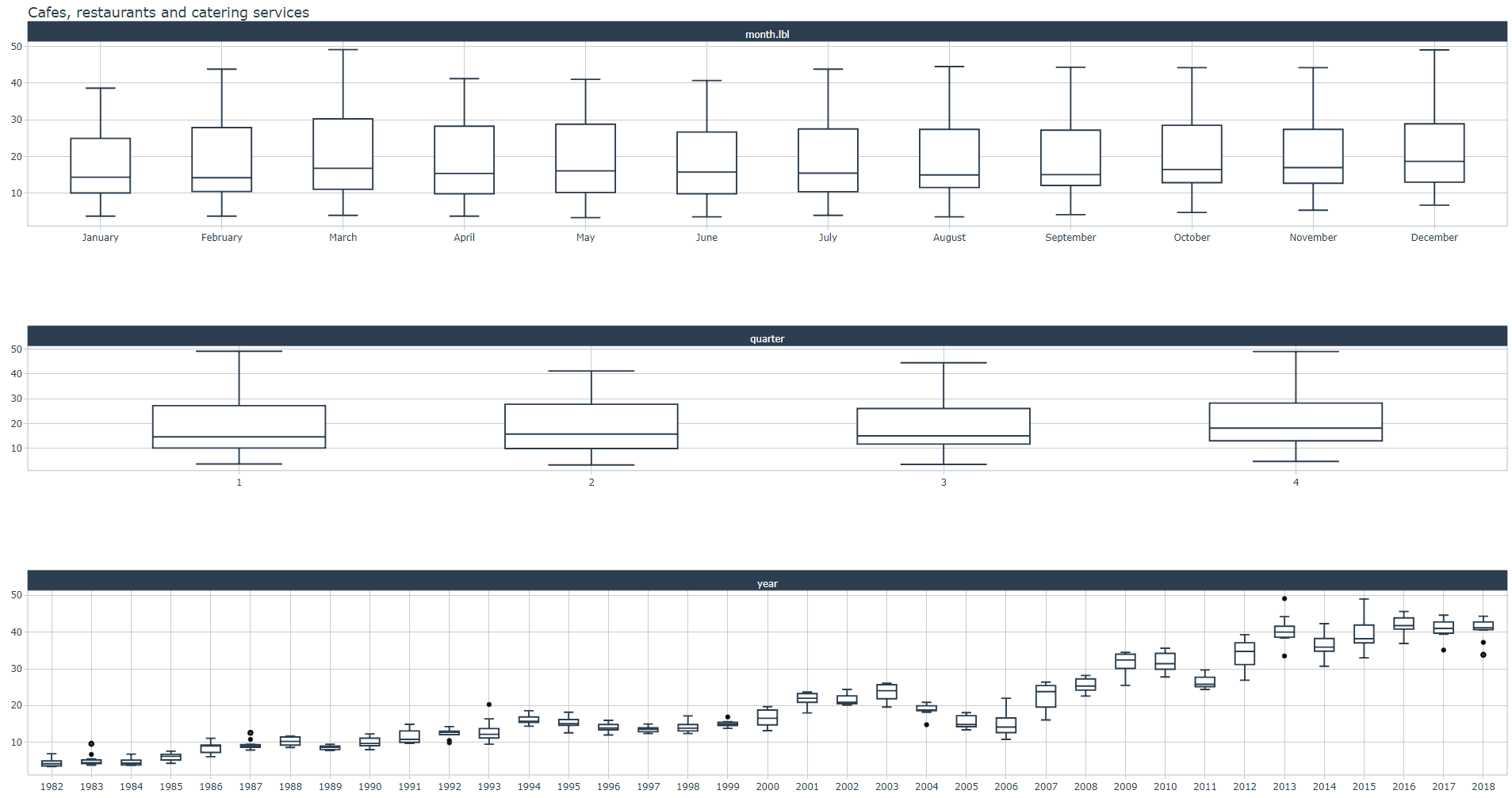
Calendar-based features
Also called Date & Time Features or Time Series Signature, these can be easily added to our monthly_retail_tbl dataset with the timetk::tk_augment_timeseries_signature() function. This function adds 25+ time series features.
industry = 1
monthly_retail_tbl %>%
  filter(Industry == Industries[industry]) %>%
  # Measure Transformation: variance reduction with Log(x+1)
  mutate(Turnover =  log1p(x = Turnover)) %>%
  # Measure Transformation: standardization
  mutate(Turnover =  standardize_vec(Turnover))
  # Add Calendar-based (or signature) features
  tk_augment_timeseries_signature(.date_var = Month) %>%
  glimpse()

Rows: 441
Columns: 31
$ Month     <date> 1982-04-01, 1982-05-01, 1982-06-01, 1982-07-01, 1982-08-01, 1982-09-01, 1982-10-01, 1982-11-01, 1982-12-01, 1983-01-01, 1983-02-01, 1983-03-01, 1983-04-01, 1983-05-0~
$ Industry  <fct> "Cafes, restaurants and catering services", "Cafes, restaurants and catering services", "Cafes, restaurants and catering services", "Cafes, restaurants and catering s~
$ Turnover  <dbl> -2.0111444, -2.3558952, -2.2810651, -2.1407005, -2.2810651, -2.0746764, -1.8908504, -1.7251364, -1.3706717, -2.2094203, -2.0746764, -2.1407005, -2.0111444, -2.0426107~
$ index.num <dbl> 386467200, 389059200, 391737600, 394329600, 397008000, 399686400, 402278400, 404956800, 407548800, 410227200, 412905600, 415324800, 418003200, 420595200, 423273600, 4~
$ diff      <dbl> NA, 2592000, 2678400, 2592000, 2678400, 2678400, 2592000, 2678400, 2592000, 2678400, 2678400, 2419200, 2678400, 2592000, 2678400, 2592000, 2678400, 2678400, 2592000, ~
$ year      <int> 1982, 1982, 1982, 1982, 1982, 1982, 1982, 1982, 1982, 1983, 1983, 1983, 1983, 1983, 1983, 1983, 1983, 1983, 1983, 1983, 1983, 1984, 1984, 1984, 1984, 1984, 1984, 1984~
$ year.iso  <int> 1982, 1982, 1982, 1982, 1982, 1982, 1982, 1982, 1982, 1982, 1983, 1983, 1983, 1983, 1983, 1983, 1983, 1983, 1983, 1983, 1983, 1983, 1984, 1984, 1984, 1984, 1984, 1984~
$ half      <int> 1, 1, 1, 2, 2, 2, 2, 2, 2, 1, 1, 1, 1, 1, 1, 2, 2, 2, 2, 2, 2, 1, 1, 1, 1, 1, 1, 2, 2, 2, 2, 2, 2, 1, 1, 1, 1, 1, 1, 2, 2, 2, 2, 2, 2, 1, 1, 1, 1, 1, 1, 2, 2, 2, 2, 2~
$ quarter   <int> 2, 2, 2, 3, 3, 3, 4, 4, 4, 1, 1, 1, 2, 2, 2, 3, 3, 3, 4, 4, 4, 1, 1, 1, 2, 2, 2, 3, 3, 3, 4, 4, 4, 1, 1, 1, 2, 2, 2, 3, 3, 3, 4, 4, 4, 1, 1, 1, 2, 2, 2, 3, 3, 3, 4, 4~
$ month     <int> 4, 5, 6, 7, 8, 9, 10, 11, 12, 1, 2, 3, 4, 5, 6, 7, 8, 9, 10, 11, 12, 1, 2, 3, 4, 5, 6, 7, 8, 9, 10, 11, 12, 1, 2, 3, 4, 5, 6, 7, 8, 9, 10, 11, 12, 1, 2, 3, 4, 5, 6, 7~
$ month.xts <int> 3, 4, 5, 6, 7, 8, 9, 10, 11, 0, 1, 2, 3, 4, 5, 6, 7, 8, 9, 10, 11, 0, 1, 2, 3, 4, 5, 6, 7, 8, 9, 10, 11, 0, 1, 2, 3, 4, 5, 6, 7, 8, 9, 10, 11, 0, 1, 2, 3, 4, 5, 6, 7,~
$ month.lbl <ord> April, May, June, July, August, September, October, November, December, January, February, March, April, May, June, July, August, September, October, November, Decemb~
$ day       <int> 1, 1, 1, 1, 1, 1, 1, 1, 1, 1, 1, 1, 1, 1, 1, 1, 1, 1, 1, 1, 1, 1, 1, 1, 1, 1, 1, 1, 1, 1, 1, 1, 1, 1, 1, 1, 1, 1, 1, 1, 1, 1, 1, 1, 1, 1, 1, 1, 1, 1, 1, 1, 1, 1, 1, 1~
$ hour      <int> 0, 0, 0, 0, 0, 0, 0, 0, 0, 0, 0, 0, 0, 0, 0, 0, 0, 0, 0, 0, 0, 0, 0, 0, 0, 0, 0, 0, 0, 0, 0, 0, 0, 0, 0, 0, 0, 0, 0, 0, 0, 0, 0, 0, 0, 0, 0, 0, 0, 0, 0, 0, 0, 0, 0, 0~
$ minute    <int> 0, 0, 0, 0, 0, 0, 0, 0, 0, 0, 0, 0, 0, 0, 0, 0, 0, 0, 0, 0, 0, 0, 0, 0, 0, 0, 0, 0, 0, 0, 0, 0, 0, 0, 0, 0, 0, 0, 0, 0, 0, 0, 0, 0, 0, 0, 0, 0, 0, 0, 0, 0, 0, 0, 0, 0~
$ second    <int> 0, 0, 0, 0, 0, 0, 0, 0, 0, 0, 0, 0, 0, 0, 0, 0, 0, 0, 0, 0, 0, 0, 0, 0, 0, 0, 0, 0, 0, 0, 0, 0, 0, 0, 0, 0, 0, 0, 0, 0, 0, 0, 0, 0, 0, 0, 0, 0, 0, 0, 0, 0, 0, 0, 0, 0~
$ hour12    <int> 0, 0, 0, 0, 0, 0, 0, 0, 0, 0, 0, 0, 0, 0, 0, 0, 0, 0, 0, 0, 0, 0, 0, 0, 0, 0, 0, 0, 0, 0, 0, 0, 0, 0, 0, 0, 0, 0, 0, 0, 0, 0, 0, 0, 0, 0, 0, 0, 0, 0, 0, 0, 0, 0, 0, 0~
$ am.pm     <int> 1, 1, 1, 1, 1, 1, 1, 1, 1, 1, 1, 1, 1, 1, 1, 1, 1, 1, 1, 1, 1, 1, 1, 1, 1, 1, 1, 1, 1, 1, 1, 1, 1, 1, 1, 1, 1, 1, 1, 1, 1, 1, 1, 1, 1, 1, 1, 1, 1, 1, 1, 1, 1, 1, 1, 1~
$ wday      <int> 5, 7, 3, 5, 1, 4, 6, 2, 4, 7, 3, 3, 6, 1, 4, 6, 2, 5, 7, 3, 5, 1, 4, 5, 1, 3, 6, 1, 4, 7, 2, 5, 7, 3, 6, 6, 2, 4, 7, 2, 5, 1, 3, 6, 1, 4, 7, 7, 3, 5, 1, 3, 6, 2, 4, 7~
$ wday.xts  <int> 4, 6, 2, 4, 0, 3, 5, 1, 3, 6, 2, 2, 5, 0, 3, 5, 1, 4, 6, 2, 4, 0, 3, 4, 0, 2, 5, 0, 3, 6, 1, 4, 6, 2, 5, 5, 1, 3, 6, 1, 4, 0, 2, 5, 0, 3, 6, 6, 2, 4, 0, 2, 5, 1, 3, 6~
$ wday.lbl  <ord> Thursday, Saturday, Tuesday, Thursday, Sunday, Wednesday, Friday, Monday, Wednesday, Saturday, Tuesday, Tuesday, Friday, Sunday, Wednesday, Friday, Monday, Thursday, ~
$ mday      <int> 1, 1, 1, 1, 1, 1, 1, 1, 1, 1, 1, 1, 1, 1, 1, 1, 1, 1, 1, 1, 1, 1, 1, 1, 1, 1, 1, 1, 1, 1, 1, 1, 1, 1, 1, 1, 1, 1, 1, 1, 1, 1, 1, 1, 1, 1, 1, 1, 1, 1, 1, 1, 1, 1, 1, 1~
$ qday      <int> 1, 31, 62, 1, 32, 63, 1, 32, 62, 1, 32, 60, 1, 31, 62, 1, 32, 63, 1, 32, 62, 1, 32, 61, 1, 31, 62, 1, 32, 63, 1, 32, 62, 1, 32, 60, 1, 31, 62, 1, 32, 63, 1, 32, 62, 1~
$ yday      <int> 91, 121, 152, 182, 213, 244, 274, 305, 335, 1, 32, 60, 91, 121, 152, 182, 213, 244, 274, 305, 335, 1, 32, 61, 92, 122, 153, 183, 214, 245, 275, 306, 336, 1, 32, 60, 9~
$ mweek     <int> 1, 1, 1, 1, 1, 1, 1, 1, 1, 1, 1, 1, 1, 1, 1, 1, 1, 1, 1, 1, 1, 1, 1, 1, 1, 1, 1, 1, 1, 1, 1, 1, 1, 1, 1, 1, 1, 1, 1, 1, 1, 1, 1, 1, 1, 1, 1, 1, 1, 1, 1, 1, 1, 1, 1, 1~
$ week      <int> 13, 18, 22, 26, 31, 35, 40, 44, 48, 1, 5, 9, 13, 18, 22, 26, 31, 35, 40, 44, 48, 1, 5, 9, 14, 18, 22, 27, 31, 35, 40, 44, 48, 1, 5, 9, 13, 18, 22, 26, 31, 35, 40, 44,~
$ week.iso  <int> 13, 17, 22, 26, 30, 35, 39, 44, 48, 52, 5, 9, 13, 17, 22, 26, 31, 35, 39, 44, 48, 52, 5, 9, 13, 18, 22, 26, 31, 35, 40, 44, 48, 1, 5, 9, 14, 18, 22, 27, 31, 35, 40, 4~
$ week2     <int> 1, 0, 0, 0, 1, 1, 0, 0, 0, 1, 1, 1, 1, 0, 0, 0, 1, 1, 0, 0, 0, 1, 1, 1, 0, 0, 0, 1, 1, 1, 0, 0, 0, 1, 1, 1, 1, 0, 0, 0, 1, 1, 0, 0, 0, 1, 1, 1, 1, 0, 0, 0, 1, 1, 0, 0~
$ week3     <int> 1, 0, 1, 2, 1, 2, 1, 2, 0, 1, 2, 0, 1, 0, 1, 2, 1, 2, 1, 2, 0, 1, 2, 0, 2, 0, 1, 0, 1, 2, 1, 2, 0, 1, 2, 0, 1, 0, 1, 2, 1, 2, 1, 2, 0, 1, 2, 0, 1, 0, 1, 2, 1, 2, 1, 2~
$ week4     <int> 1, 2, 2, 2, 3, 3, 0, 0, 0, 1, 1, 1, 1, 2, 2, 2, 3, 3, 0, 0, 0, 1, 1, 1, 2, 2, 2, 3, 3, 3, 0, 0, 0, 1, 1, 1, 1, 2, 2, 2, 3, 3, 0, 0, 0, 1, 1, 1, 1, 2, 2, 2, 3, 3, 0, 0~
$ mday7     <int> 1, 1, 1, 1, 1, 1, 1, 1, 1, 1, 1, 1, 1, 1, 1, 1, 1, 1, 1, 1, 1, 1, 1, 1, 1, 1, 1, 1, 1, 1, 1, 1, 1, 1, 1, 1, 1, 1, 1, 1, 1, 1, 1, 1, 1, 1, 1, 1, 1, 1, 1, 1, 1, 1, 1, 1~
We must normalize index.num and year columns, and we can suppress redundant and useless columns such as year.iso, month.xts and diff.
Since we are dealing with monthly data, all hourly-, daily- and weekly-related columns can be suppressed.
All categorical variables can be dummyfied, this is the case for month.lbl column which can be removed after being one-hot encoded.
You can glimpse() the preprocesing pipe to display remaining features which will become the predictors of the subsequent linear regression function (plot_time_series_regression()).
Run the linear regression, check adjusted R-squared value and corresponding fit plot. Notice that you must add the month. prefix to each predictor in the linear regression .formula.
industry = 1
monthly_retail_tbl %>%
  filter(Industry == Industries[industry]) %>%

  # Measure Transformation: variance reduction with Log(x+1)
  mutate(Turnover =  log1p(x = Turnover)) %>%
  # Measure Transformation: standardization
  mutate(Turnover =  standardize_vec(Turnover))

  # Add Calendar-based (or signature) features
  tk_augment_timeseries_signature(.date_var = Month) %>%monthly_retail_tbl %>%
  select(-diff, -matches("(.xts$)|(.iso$)|(hour)|(minute)|(second)|(day)|(week)|(am.pm)")) %>%
  dummy_cols(select_columns = c("month.lbl")) %>%
  select(-month.lbl) %>%
  mutate(index.num = normalize_vec(x = index.num)) %>%
  mutate(year = normalize_vec(x = year)) %>%

  # Perfom linear regression
  plot_time_series_regression(.date_var = Month,
                              .formula = Turnover ~ as.numeric(Month) +
                                index.num + year + half + quarter + month +
                                month.lbl_January + month.lbl_February + month.lbl_March + month.lbl_April +
                                month.lbl_May + month.lbl_June + month.lbl_July + month.lbl_August +
                                month.lbl_September + month.lbl_October + month.lbl_November + month.lbl_December,
                              .show_summary = TRUE)
Adjusted R-squared: 0.9028
Fourier terms features
As per 3, "With Fourier terms, we often need fewer predictors than with dummy variables. If m is the seasonal period, then the first few Fourier terms are given by
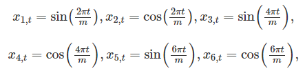
and so on. .K specifies how many pairs of sin and cos terms to include". Note: "A regression model containing Fourier terms is often called a harmonic regression".
After experimenting with several combinations of m and K values, I've decided to set m = 12 (1-year period) and K = 1. Notice that we need to add the Month_ to the corresponding predictor within linear regression formula.
Run the code snippet below to see how the Fourier terms look like
monthly_retail_tbl %>%
  filter(Industry == Industries[industry]) %>%
  mutate(Turnover =  log1p(x = Turnover)) %>%
  mutate(Turnover =  standardize_vec(Turnover)) %>%
  tk_augment_fourier(.date_var = Month, .periods = 12, .K = 1) %>%
  select(-Industry) %>%
  pivot_longer(-Month) %>%
  plot_time_series(Month, .value = value,
                   .facet_vars = name,
                   .smooth = FALSE)

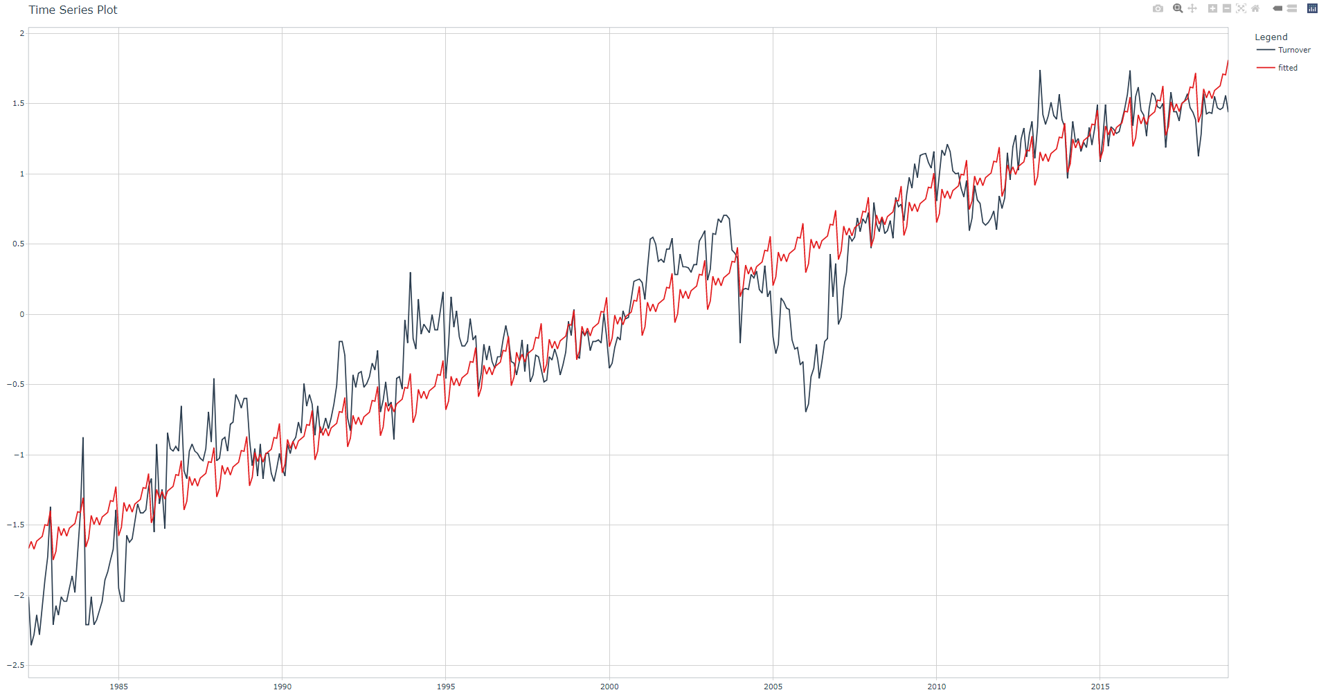
Run the linear regression, check adjusted R-squared value and corresponding fit plot.
industry = 1
monthly_retail_tbl %>%
  filter(Industry == Industries[industry]) %>%

  # Measure Transformation: variance reduction with Log(x+1)
  mutate(Turnover =  log1p(x = Turnover)) %>%
  # Measure Transformation: standardization
  mutate(Turnover =  standardize_vec(Turnover))

  # Add Calendar-based (or signature) features
  tk_augment_timeseries_signature(.date_var = Month) %>%monthly_retail_tbl %>%
  select(-diff, -matches("(.xts$)|(.iso$)|(hour)|(minute)|(second)|(day)|(week)|(am.pm)")) %>%
  dummy_cols(select_columns = c("month.lbl")) %>%
  select(-month.lbl) %>%
  mutate(index.num = normalize_vec(x = index.num)) %>%
  mutate(year = normalize_vec(x = year)) %>%

  # Add Fourier features
  tk_augment_fourier(.date_var = Month, .periods = 12, .K = 1) %>%

  # Perfom linear regression
  plot_time_series_regression(.date_var = Month,
                              .formula = Turnover ~ as.numeric(Month) +
                                index.num + year + half + quarter + month +
                                month.lbl_January + month.lbl_February + month.lbl_March + month.lbl_April +
                                month.lbl_May + month.lbl_June + month.lbl_July + month.lbl_August +
                                month.lbl_September + month.lbl_October + month.lbl_November + month.lbl_December +
                                Month_sin12_K1 + Month_cos12_K1,
                              .show_summary = TRUE)
Adjusted R-squared: 0.9037.
Lag features
As per 1, “Lag features are values at prior timesteps that are considered useful because they are created on the assumption that what happened in the past can influence or contain a sort of intrinsic information about the future.”
Below, two zoomed plots with the PACF for the first and third industry:
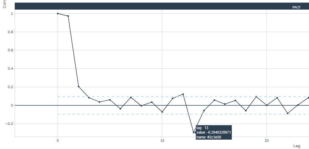
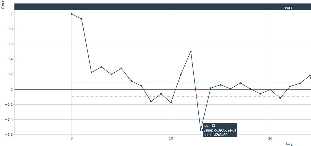
Generally (for all industries), highest statistical significance are located at lags 12 and 13. After experimenting with other lag values, I've decided to set both the 12- and 13-month lags. Notice that we need to add the Turnover_ to the corresponding predictor within linear regression formula. Clearly, 12 NA values will be present at the begining of the Turnover_lag12 and Turnover_lag13 columns.
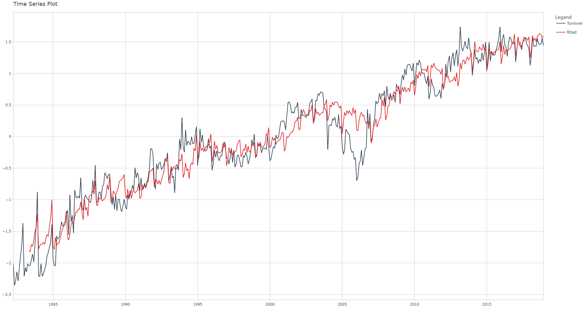
Run the linear regression, check adjusted R-squared value and corresponding fit plot. Important: linear regression is based on the famous lm() which automatically ignores all rows with NA.
industry = 1
monthly_retail_tbl %>%
  filter(Industry == Industries[industry]) %>%
  mutate(Turnover =  log1p(x = Turnover)) %>%
  mutate(Turnover =  standardize_vec(Turnover)) %>%
  tk_augment_timeseries_signature(.date_var = Month) %>%
  select(-diff, -matches("(.xts$)|(.iso$)|(hour)|(minute)|(second)|(day)|(week)|(am.pm)")) %>%
  dummy_cols(select_columns = c("month.lbl")) %>%
  select(-month.lbl) %>%
  mutate(index.num = normalize_vec(x = index.num)) %>%
  mutate(year = normalize_vec(x = year)) %>%
  tk_augment_fourier(.date_var = Month, .periods = 12, .K = 1) %>%
  tk_augment_lags(.value = Turnover, .lags = c(12, 13)) %>%
  plot_time_series_regression(.date_var = Month,
                              .formula = Turnover ~ as.numeric(Month) +
                                index.num + year + half + quarter + month +
                                month.lbl_January + month.lbl_February + month.lbl_March + month.lbl_April +
                                month.lbl_May + month.lbl_June + month.lbl_July + month.lbl_August +
                                month.lbl_September + month.lbl_October + month.lbl_November + month.lbl_December +
                                Month_sin12_K1 + Month_cos12_K1 +
                                Turnover_lag12 + Turnover_lag13,
                              .show_summary = TRUE)
Adjusted R-squared: 0.9237
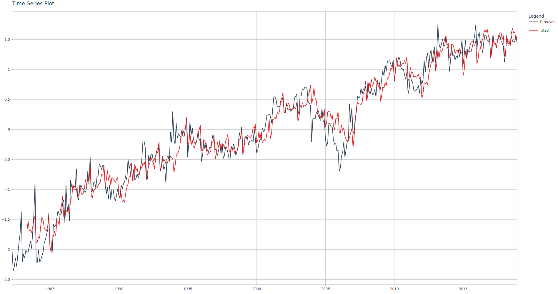
Rolling Lags features
As per 1,“The main goal of building and using rolling window statistics in a time series dataset is to compute statistics on the values from a given data sample by defining a range that includes the sample itself as well as some specified number of samples before and after the sample used.”
After experimenting with several rolling period values, I've decided to set three rolling periods: 3-, 6- and 12-month periods. The mean will be calculated condering a center alignment. We set the .partial parameter to TRUE. Since the first 12 values of Turnover_lag12 are NA, other NA and NaN values will be present in corresponding rolling lags features. Run ?tk_augment_slidify for more information.
This is how the rolling lags look like
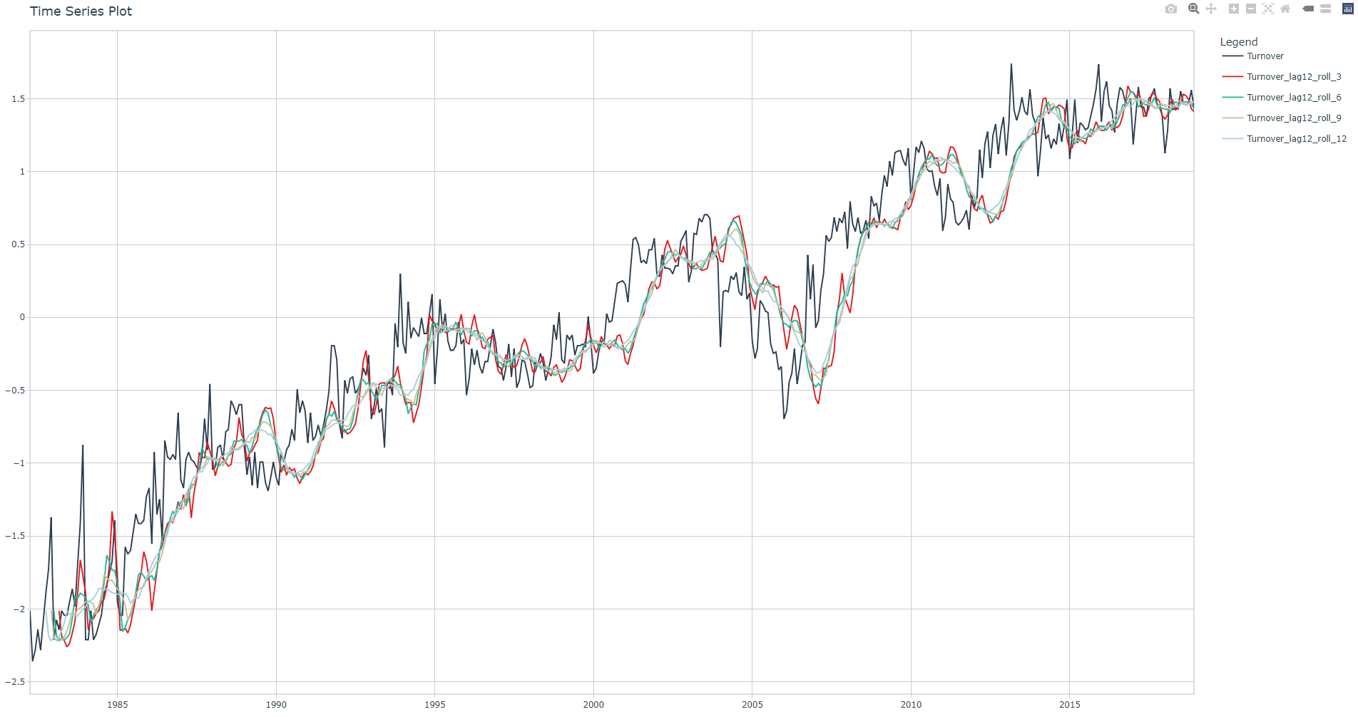
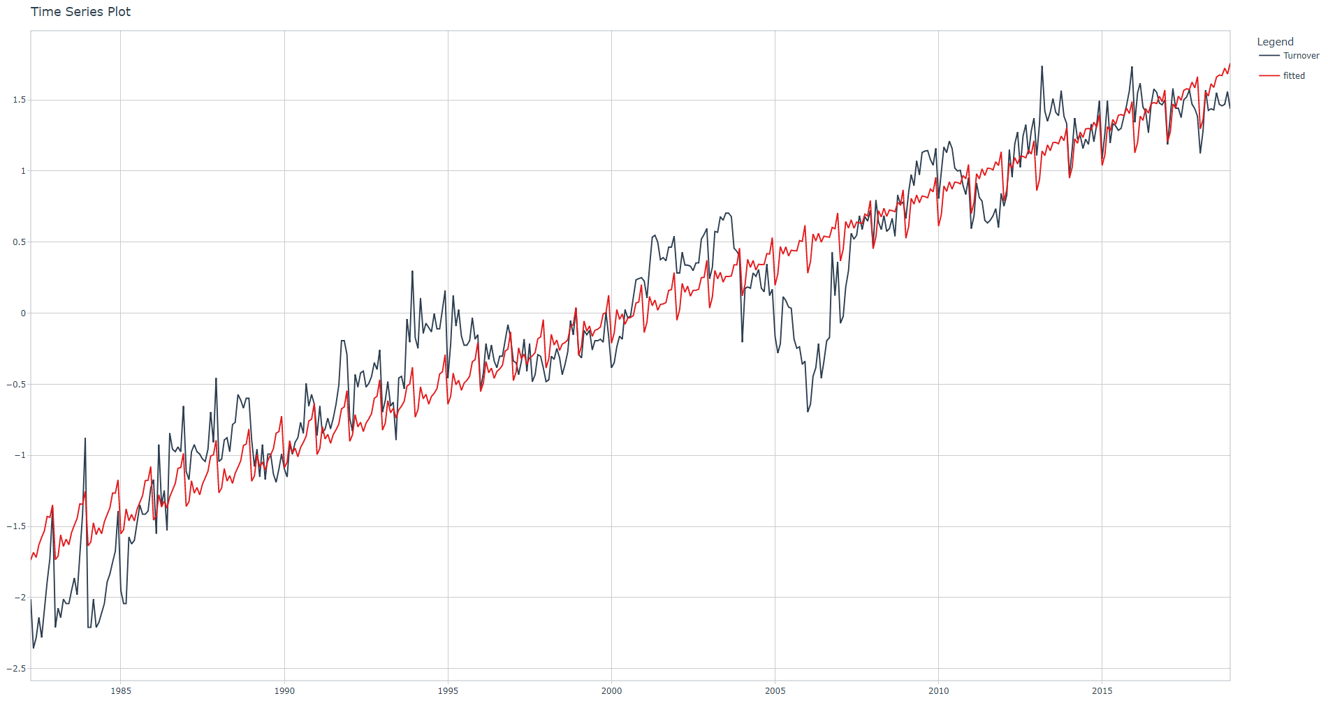
Run the linear regression, check adjusted R-squared value and corresponding fit plot.
Adjusted R-squared: 0.9481. R-squared have been improved. Please note that rolling lags features can be very helpful for some machine learning algorithms. This has been demonstrated in contests such as M5 .
I have also included the linear regression summary, notice how some Fourier and Rolling Lags features are statistically significant (** or ***).
monthly_retail_tbl %>%
  filter(Industry == Industries[industry]) %>%
  mutate(Turnover =  log1p(x = Turnover)) %>%
  mutate(Turnover =  standardize_vec(Turnover)) %>%
  tk_augment_timeseries_signature(.date_var = Month) %>%
  select(-diff, -matches("(.xts$)|(.iso$)|(hour)|(minute)|(second)|(day)|(week)|(am.pm)")) %>%
  dummy_cols(select_columns = c("month.lbl")) %>%
  select(-month.lbl) %>%
  mutate(index.num = normalize_vec(x = index.num)) %>%
  mutate(year = normalize_vec(x = year)) %>%
  tk_augment_fourier(.date_var = Month, .periods = 12, .K = 1) %>%
  tk_augment_lags(.value = Turnover, .lags = c(12, 13)) %>%
  tk_augment_slidify(.value   = c(Turnover_lag12, Turnover_lag13),
                     .f       = ~ mean(.x, na.rm = TRUE),
                     .period  = c(3, 6, 9, 12),
                     .partial = TRUE,
                     .align   = "center") %>%
  plot_time_series_regression(.date_var = Month,
                              .formula = Turnover ~ as.numeric(Month) +
                                index.num + year + half + quarter + month +
                                month.lbl_January + month.lbl_February + month.lbl_March + month.lbl_April +
                                month.lbl_May + month.lbl_June + month.lbl_July + month.lbl_August +
                                month.lbl_September + month.lbl_October + month.lbl_November + month.lbl_December +
                                Month_sin12_K1 + Month_cos12_K1 +
                                Turnover_lag12 + Turnover_lag12_roll_3  + Turnover_lag12_roll_6  + Turnover_lag12_roll_9 + Turnover_lag12_roll_12 +
                                Turnover_lag13 + Turnover_lag13_roll_3  + Turnover_lag13_roll_6  + Turnover_lag13_roll_9 + Turnover_lag13_roll_12,
                              .show_summary = TRUE)

Call:
stats::lm(formula = .formula, data = df)

Residuals:
     Min       1Q   Median       3Q      Max
-0.65228 -0.12624 -0.00067  0.13133  0.78657

Coefficients: (5 not defined because of singularities)
                        Estimate Std. Error t value Pr(>|t|)
(Intercept)             95.30640  163.30413   0.584  0.55981
as.numeric(Month)       -0.02211    0.03753  -0.589  0.55606
index.num                     NA         NA      NA       NA
year                   291.82727  493.48550   0.591  0.55461
half                     0.14258    0.11774   1.211  0.22661
quarter                 -0.16283    0.18058  -0.902  0.36775
month                    0.75295    1.12805   0.667  0.50485
month.lbl_January        0.20144    0.18917   1.065  0.28758
month.lbl_February       0.18250    0.13264   1.376  0.16961
month.lbl_March          0.16548    0.10107   1.637  0.10235
month.lbl_April          0.14551    0.15349   0.948  0.34368
month.lbl_May            0.10645    0.10276   1.036  0.30086
month.lbl_June                NA         NA      NA       NA
month.lbl_July           0.05333    0.16037   0.333  0.73963
month.lbl_August         0.05699    0.09385   0.607  0.54407
month.lbl_September           NA         NA      NA       NA
month.lbl_October        0.12642    0.11781   1.073  0.28388
month.lbl_November            NA         NA      NA       NA
month.lbl_December            NA         NA      NA       NA
Month_sin12_K1          -0.05217    0.01766  -2.953  0.00333 **
Month_cos12_K1          -0.05522    0.01798  -3.071  0.00228 **
Turnover_lag12           0.15671    0.19215   0.816  0.41521
Turnover_lag12_roll_3    0.20053    0.38534   0.520  0.60307
Turnover_lag12_roll_6    0.36903    0.43344   0.851  0.39505
Turnover_lag12_roll_9   -0.79671    0.74807  -1.065  0.28750
Turnover_lag12_roll_12   4.55934    0.58574   7.784 6.01e-14 ***
Turnover_lag13           0.07664    0.19488   0.393  0.69434
Turnover_lag13_roll_3   -0.17368    0.34252  -0.507  0.61239
Turnover_lag13_roll_6   -0.43496    0.56519  -0.770  0.44199
Turnover_lag13_roll_9   -1.43135    0.60602  -2.362  0.01866 *
Turnover_lag13_roll_12  -1.87214    0.73649  -2.542  0.01140 *
---
Signif. codes:  0 ‘***’ 0.001 ‘**’ 0.01 ‘*’ 0.05 ‘.’ 0.1 ‘ ’ 1

Residual standard error: 0.2159 on 402 degrees of freedom
  (13 observations deleted due to missingness)
Multiple R-squared:  0.9511,    Adjusted R-squared:  0.9481
F-statistic: 312.9 on 25 and 402 DF,  p-value: < 2.2e-16
Conclusion
In this article I have introduced the time series feature engineering step through an exploratory method consisting in running a linear regression and checking the adjusted R-squared each time we add common features such as calendar-based, lags, rolling lags, and Fourier terms.
Needless to say that setting Fourier m and K values, lag period value, and rolling period values required experimentation, checking the R-squared for each setting.
You have noticed how the adjusted R-squared (proportion of the variance explained by the linear regression model) increased by adding these common features which means that they can be are very helpful as predictors. Illustrations show results for a single Industry value but you can display the same results for other Industry values.
In the next article (Part2) I explain the official feature engineering method by using recipes; a recipe will be added along with a machine learning model to a workflow which is fundamental for the understanding of the modeltime package (Part 3).
References
1 Lazzeri, Francesca "Introduction to feature engineering for time series forecasting", Medium, 10/5/2021
2 Dancho, Matt, "DS4B 203-R: High-Performance Time Series Forecasting", Business Science University
3 Hyndman R., Athanasopoulos G., "Forecasting: Principles and Practice", 3rd edition