Quantum Entanglement
Multiple systems - Principles and examples

Cover photo by inkoly ref. 1185114379 on iStock
Go to R-bloggers for R news and tutorials contributed by hundreds of R bloggers.
This is the second article of the Quantum Computing simulation with R series.
Introduction
Welcome back to our quantum journey! Today, we're delving into a phenomenon that lies at the heart of quantum computing's unique power - entanglement. At a high level, quantum entanglement is the deep and mysterious link that can exist between two qubits, no matter the distance that separates them. This powerful feature allows quantum computers to process a massive number of possibilities at once and solve certain problems much faster than classical computers.
But how do we get there? We'll start by exploring two-qubit gates, the essential quantum operations that can bring about entanglement. The most common of these gates, such as the CNOT gate, can modify the state of one qubit based on the state of another, creating a correlation between the two.
Next, we'll dive into the concept of the tensor product. When dealing with multiple qubits, we cannot simply consider them separately; we must take into account the joint system, described mathematically by the tensor product of the individual states. In some situations, the state of the whole system cannot be described by individual qubit states, and that's when we encounter true entanglement.
We'll contrast this with the notion of product states, which do not involve entanglement. In these cases, the state of the whole system can be factored into individual qubit states. However, the fascinating aspect of quantum systems is that product states and entangled states are not mutually exclusive categories; a quantum state can evolve from one to the other under the action of certain quantum gates.
Entanglement is a key resource in quantum computing and quantum information theory, as it is a prerequisite for quantum teleportation, quantum cryptography, superdense coding, and several types of quantum computing algorithms. The phenomenon of quantum entanglement allows quantum computers to perform complex calculations in parallel, providing them with immense computational power. However, managing and maintaining entanglement remains one of the main challenges in the practical implementation of quantum computing.
Get ready to delve into these deep waters where classical intuition may fall short, but a new, broader understanding awaits.
What is quantum entanglement?
Quantum entanglement is a profound physical phenomenon that occurs when a pair or a group of quantum particles interact in a way that the state of each particle cannot be described independently of the state of the others, regardless of the distance separating them. This implies that an alteration in the state of one entangled particle instantaneously affects the state of the other particle(s), no matter how far apart they are. This counterintuitive feature stems from the principles of quantum mechanics, notably the superposition principle.
In more technical terms, an entangled state cannot be factorized as a product of the states of its constituents; that is, it cannot be broken down into separate states for each particle.
Superposition and entanglement are two distinct concepts in quantum mechanics.
Superposition refers to the fact that a quantum state can exist in multiple states at once. For example, a qubit could be in a superposition of the states |0⟩ and |1⟩, represented as α|0⟩ + β|1⟩, where α and β are complex numbers and |α|^2 + |β|^2 = 1. Superposition can occur with a single qubit.
Entanglement refers to a special correlation that can exist between quantum states. When two qubits are entangled, the state of one qubit is immediately connected to the state of the other, no matter the distance between them. Entanglement is a property of a system of two or more qubits.
How do we create an entangled quantum state?
Although I have not introduced the CNOT gate yet, it is good to know why we apply it in the following example.
Example:
Start with a separable state, say |00⟩
Apply Hadamard gate to the first qubit: 1/√2 (|00⟩ + |10⟩)
Apply CNOT gate => 1/√2 (|00⟩ + |11⟩) is an entangled state
Let us perform these steps with the qsimulatR package
# Create qstate object |00>
> x <- qstate(nbits = 2)
> x
   ( 1 )    * |00>
# Display superposition of bit 1 of |00> (the rightmost qubit)
# with the Hadamard gate
> H(1)*x
   ( 0.7071068 )    * |00>
 + ( 0.7071068 )    * |01>
# Apply CNOT gate
> x <- CNOT(c(1,2))*(H(1)*x)
# control bit = bit 1, target bit (t) = bit 2
> x
   ( 0.7071068 )    * |00> # control = 0 then target = 0
 + ( 0.7071068 )    * |11> # control = 1 then target = 1
# Verify result with CNOT truth table
> truth.table(CNOT, nbits = 2)
  In2 In1 Out2 Out1
1   0   0    0    0 # CNOT(I00>) = |00>
2   0   1    1    1 # CNOT(|01>) = |11>
3   1   0    1    0
4   1   1    0    1
There are two notions here that were not included in my first article: the CNOT gate and a separable state.
The CNOT (Controlled-NOT) gate
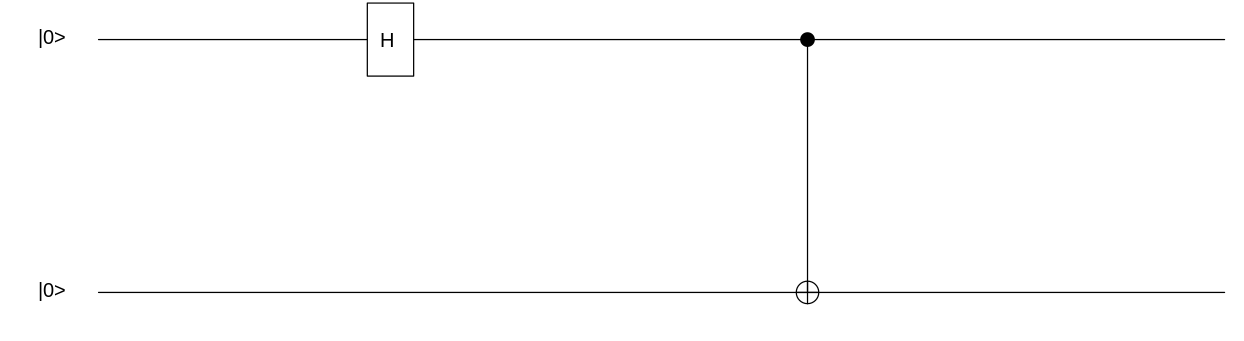
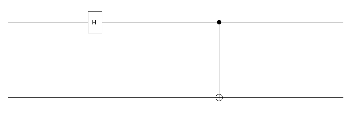
Let us start by plotting the circuit of the previous result.
# qubitnames = c("|0>", "|0>") since we started with |00>
> qsimulatR::plot(x, qubitnames = c("|0>", "|0>"))
The Controlled-Not gate (CNot, controlled-X, CX, Feynman) is typically represented by the circuit diagrams [1]
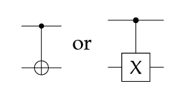
The control bit • influences the state of the target bit ⊕, and the target bit has no influence on the state of the control bit e.g. it is not symmetric between the two qubits.
The gate flips (or NOTs) the target qubit if the control qubit is in state |1⟩, as shown in the CNOT truth table above where In1 is the control bit and In2 is the target bit.
The state of the target qubit becomes entangled with the control qubit, which means that the state of the control qubit is now related to the state of the target qubit (the back reaction).
This concept of "action and back reaction" is a reflection of the principle of entanglement in quantum mechanics, and the foundation of quantum gates being reversible e.g. if we know the final state of the two qubits, we can figure out their initial state.
In quantum computing, every operation is required to be reversible, meaning if we know the output state, we can exactly figure out the input state.
# the first bit is the control and the second bit the target.
> CNOT(c(1,2))
An object of class "cnotgate"
Slot "bits":
[1] 1 2
# you can switch the control and atrget bits
> CNOT(c(2,1))
An object of class "cnotgate"
Slot "bits":
[1] 2 1

> x <- qstate(nbits = 2)
> qsimulatR::plot(CNOT(c(2,1))*(H(2)*x), qubitnames = c("|0>", "|0>"))
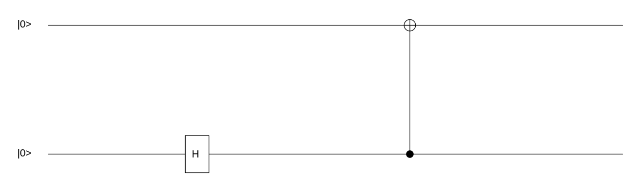
In quantum logic, there are no pure control operations per se. There is no unambiguous distinction between control and target [1]. This means that after a CNOT operation, neither qubit can be said to have a purely "control" or "target" role because their states are intertwined - each qubit's state depends on the other's.
Now, what do we mean by separable qubit?
Product states
In quantum mechanics, a state is separable (or is a product state) if it can be written as a product of states of individual subsystems.
For a two-qubit system, a state is separable if it can be written in the form |ψ⟩ = |a⟩ ⊗ |b⟩, where |a⟩ and |b⟩ are states of the individual qubits, and ⊗ is the tensor product.
For instance, |00⟩, |01⟩, |10⟩, and |11⟩ are all separable states.
If you can factor the state into a product of two single-qubit states then the state is separable. If you can't, then the state is entangled.
For instance, the state α|00⟩ + β|11⟩ cannot be factored into a product of two single-qubit states unless either α or β is zero. Therefore, this state is entangled.
Tensor product
Tensor products of quantum state vectors are also quantum state vectors — and they represent independence among systems.
The tensor product |φ⟩⊗|ψ⟩ may alternatively be written as |φ⟩|ψ⟩ or as |φψ⟩.
$$|0>⊗|1> = \begin{pmatrix} 1 \\ 0 \end{pmatrix} ⊗ \begin{pmatrix} 0 \\ 1 \end{pmatrix} = \begin{pmatrix} 0 \\ 1 \\ 0 \\ 0 \end{pmatrix} = |01>$$
You can compute the tensor product between two quantum state vectors by applying the kronecker() function in R to qstate coefs.
> a <- qstate(1) # |0>
> b <- X(1)*a    # |1>
> kronecker(a@coefs, b@coefs)
[1] 0+0i 1+0i 0+0i 0+0i
> ab <- qstate(2, coefs = kronecker(a@coefs, b@coefs))
> ab
   ( 1 )    * |01>
Proving entanglement with CNOT gates
Based on the example provided in Chapter 2.1.10 from the book [2] by Bourreau et al., I am going to implement the detailed computation with the qsimulatR package. I hope you will get another sense of what entanglement means.
We start with two qubits
$$|x1>= \begin{pmatrix} 0.8 \\ 0.6 \end{pmatrix} \hspace{1cm} |x2>= \begin{pmatrix} 0.38 \\ 0.92 \end{pmatrix}$$
After applying the first CNOT gate we obtain
$$|x1>= \begin{pmatrix} 0.8 \\ 0.6 \end{pmatrix} \hspace{1cm} |x2>= \begin{pmatrix} 0.63 \\ 0.77 \end{pmatrix}$$
After applying the second CNOT gate we obtain
$$|x1>= \begin{pmatrix} 0.8 \\ 0.6 \end{pmatrix} \hspace{1cm} |x2>= \begin{pmatrix} 0.683 \\ 0.721 \end{pmatrix}$$
# Helper function: probabilities of a quantum state
qstateProbabilities <- function(x){
  probs <- Mod(z = x@coefs)^2
  names(probs) <- x@basis
  return(probs)
}

# qubit |x1>
> x1 <- qstate(1, coefs = as.complex(c(.8, .6)))
> x1
   ( 0.8 )    * |0>
 + ( 0.6 )    * |1>
> qstateProbabilities(x1)
 |0>  |1>
0.64 0.36
# qubit |x2>
> x2 <- qstate(1, coefs = as.complex(c(5/13, 12/13)))
> x2
   ( 0.3846154 )    * |0>
 + ( 0.9230769 )    * |1>
>
> qstateProbabilities(x2)
     |0>      |1>
0.147929 0.852071
Let us perform the tensor product |x1>⊗ |x2> = |x1x2> with the kronecker() function.
# quantum state |x1x2>
> x1x2 <- qstate(2, coefs = as.complex(kronecker(x1@coefs, x2@coefs)))
> x1x2
   ( 0.3076923 )    * |00>
 + ( 0.7384615 )    * |01>
 + ( 0.2307692 )    * |10>
 + ( 0.5538462 )    * |11>
Now we apply the first CNOT gate and compute the probabilities for both qubits, |x1> and |x2>, to be in states |0> and |1>, respectively.
# First CNOT : CNOT(|x1x2>)
# x1 is the control bit thus bit 2
# x2 is the target bit thus bit 1
> res <- CNOT(c(2,1))*x1x2
> res
   ( 0.3076923 )    * |00>
 + ( 0.7384615 )    * |01>
 + ( 0.5538462 )    * |10>
 + ( 0.2307692 )    * |11>
> probs <- qstateProbabilities(res)
> probs
      |00>       |01>       |10>       |11>
0.09467456 0.54532544 0.30674556 0.05325444

# Prob(x1=|0>) => unchanged
> as.numeric(probs[1]+probs[2])
[1] 0.64
# Prob(x1=|1>) => unchanged
> as.numeric(probs[3]+probs[4])
[1] 0.36
# Prob(x2=|0>) => updated to 0.4014201 > 0.147929
> as.numeric(probs[1]+probs[3])
[1] 0.4014201
# Prob(x2=|1>) => updated to 0.5985799 < 0.852071
> as.numeric(probs[2]+probs[4])
[1] 0.5985799
This means that we obtain an updated |x2> with updated probabilities, we compute its coefficients knowing that coef = √prob. Consequently, we obtain an updated quantum state |x1>⊗ |x2> = |x1x2>
# Updated |x2>
> x2 <- qstate(nbits = 1,
               coefs = as.complex(c(sqrt(probs[1]+probs[3]),
                                    sqrt(probs[2]+probs[4]))))
> x2
   ( 0.6335772 )    * |0>
 + ( 0.7736794 )    * |1>
# Thus, quantum state |x1x2> is now
> x1x2 <- qstate(2, coefs = as.complex(kronecker(x1@coefs, x2@coefs)))
> x1x2
   ( 0.5068618 )    * |00>
 + ( 0.6189436 )    * |01>
 + ( 0.3801463 )    * |10>
 + ( 0.4642077 )    * |11>
Now we apply the second CNOT gate and compute the probabilities for both qubits, |x1> and |x2>, to be in states |0> and |1>, respectively.
# Second CNOT : CNOT(|x1x2>)
# x1 is the control bit thus bit 2
# x2 is the target bit thus bit 1
> res <- CNOT(c(2,1))*x1x2
> res
   ( 0.5068618 )    * |00>
 + ( 0.6189436 )    * |01>
 + ( 0.4642077 )    * |10>
 + ( 0.3801463 )    * |11>
> probs <- qstateProbabilities(res)
> probs
     |00>      |01>      |10>      |11>
0.2569089 0.3830911 0.2154888 0.1445112
# Prob(x1=|0>) => unchanged
> as.numeric(probs[1]+probs[2])
[1] 0.64
# Prob(x1=|1>) => unchanged
> as.numeric(probs[3]+probs[4])
[1] 0.36
# Prob(x2=|0>) => updated to 0.4723976 > 0.4014201 > 0.147929
> as.numeric(probs[1]+probs[3])
[1] 0.4723976
# Prob(x2=|1>) => updated to 0.5276024 < 0.5985799 < 0.852071
> as.numeric(probs[2]+probs[4])
[1] 0.5276024
As before, we obtain an updated |x2> with updated probabilities, we compute its coefficients knowing that coef = √prob.
# Updated |x2>
> x2
   ( 0.6873119 )    * |0>
 + ( 0.7263624 )    * |1>
Thus,
the probability of (|x2> = |0>) increased from 0.15 to 0.47
the probability of (|x2> = |1>) decreased from 0.85 to 0.53
And there is a reason for this! indeed, the (unchanged) probability of (|x1> = |1>) = 0.36 < 0.5 thus, |x1> is closer to state |0>. This means that applying the CNOT several times, with x1 as the control bit and x2 as the target bit, will make |x2> to converge to state |0> as well => entanglement!
Bell states
Remember the entangled state 1/√2 (|00⟩ + |11⟩) from the very first example in this article? it is called a Bell state.
All four of the Bell states represent entanglement between two qubits [3].
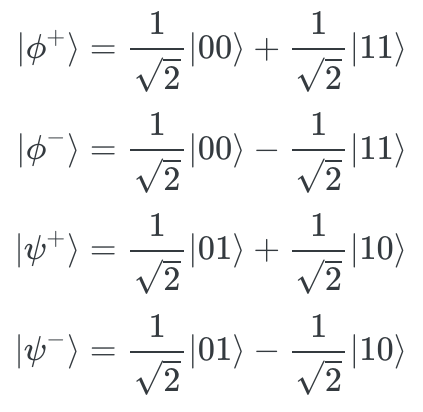
The collection of all four Bell states is known as the Bell basis. Any quantum state vector of two qubits can be expressed as a linear combination of the four Bell states [3]. For example,
$$|00> =\frac{1}{\sqrt{2}}|\phi^+> + \frac{1}{\sqrt{2}}|\phi^->$$
> x <- qstate(2) # |00>
> x <- CNOT(c(1,2))*(H(1)*x)
# Bell state |phi+>
> x
   ( 0.7071068 )    * |00> # control = 0 then target = 0
 + ( 0.7071068 )    * |11> # control = 1 then target = 1
# Try it with x = {|01>, |10>, |11>}
# I guess you have understood how we obtain the Bell states now
qsimulatR::plot(x)
References
[1] Crooks G. E., "Gates, States, and Circuits", Tech. Note 014v0.9.0 beta, 2023-03-01
[2] Bourreau E., Fleury, G., Lacomme P., "Introduction à l'informatique quantique, Apprendre à calculer sur des ordinateurs quantiques avec Python", Collection Blanche, Eyrolles, 2022
[3] Qiskit, Basics of Quantum Information, https://learn.qiskit.org/course/basics/single-systems