

Cover photo by berya113 ref. 1126414116 on iStock
Go to R-bloggers for R news and tutorials contributed by hundreds of R bloggers.
This is the first article of the Quantum Computing simulation with R series.
Welcome to our series on quantum computing basics with the qsimulatR package. This is the first in a series of articles aimed at providing an accessible and practical introduction to the basics of quantum computing using the R language. If you are a beginner in quantum computing but have a working knowledge of R, you're in the right place!
Introduction
qsimulatR is a quantum computer simulator developed by Ostmeyer and Urbach [1], it provides an excellent package to learn, explore, and experiment with quantum computing basics in the comfort of the R programming environment. Not only does it simulate the behavior of a quantum computer, but it also allows you to construct quantum circuits, perform computations and convert the code to Qiskit, making it a powerful tool for quantum computing beginners.
In this article, we will explore single-system quantum states, delve into the concept of superposition, calculate state probabilities, and understand what happens during a quantum measurement. Along the way, we will also learn about essential quantum gates such as the Hadamard gate, Pauli gates (X, Z, Y), and Phase gates (S, T), as well as their geometric interpretations with the Bloch sphere.
While the qsimulatR package provides a succinct explanation in its vignette document [2], our goal in this series is to expand on these foundations and present them in a more beginner-friendly manner. We will make use of numerous examples, code snippets, and visual aids, all aimed at making your quantum computing journey more manageable and enjoyable.
So let's set off on this exciting journey of discovery into the world of quantum computing. Prepare to leave your classical computation instincts behind and enter a realm where seemingly impossible tasks become possible!
Quantum States
The term qubit (quantum bit) refers to a quantum system whose classical state set is {0, 1}. It is just a bit, but it can be in a quantum state [3].
A quantum state of a system is represented by a column vector characterized by these two properties:
The entries of a quantum state vector are complex numbers.
The sum of the absolute values squared of the entries of a quantum state vector must be equal to 1.
For a single qubit, the computational basis consists of two states: |0⟩ and |1⟩. These basis states are orthogonal, meaning they are independent of each other and can't be created by combining the other.
Thus, the following are the vectors of states |0⟩ and |1⟩ respectively,
$$\begin{pmatrix} 1 \\ 0 \\ \end{pmatrix} = |0> , \begin{pmatrix} 0 \\ 1 \\ \end{pmatrix} = |1>$$
Let us define |0> with the qsimulatR package:
> ket0 <- qstate(nbits = 1)
> ket0
 ( 1 )    * |0>
Let us now look at the structure of the |0> qstate object
> str(ket0)
Formal class 'qstate' [package "qsimulatR"] with 5 slots
  ..@ nbits  : int 1
  ..@ coefs  : cplx [1:2] 1+0i 0+0i
  ..@ basis  : chr [1:2] "|0>" "|1>"
  ..@ noise  :List of 4
  .. ..$ p    : num 0
  .. ..$ bits : int 1
  .. ..$ error: chr "any"
  .. ..$ args : list()
  ..@ circuit:List of 2
  .. ..$ ncbits  : num 0
  .. ..$ gatelist: list()
The values of the coefs slot confirm that |0> is indeed a vector with two complex entries (1, 0) = (1+0i, 0+0i).
Let us do the same thing for |1>. We can define |1> by explicitly creating the qstate object with coefficient vector (0, 1) or by applying a bit flip with an X gate to |0> (recommended). The Pauli X gate will be explained later in this chapter.
# create |1> with coefficient vector (0, 1).
> ket1 <- qstate(nbits = 1, coefs = c(0, 1))
> ket1
   ( 1 )    * |1>

# apply bit flip with an X gate to |0> (recommended)
> ket1 <- X(1)*ket0
> ket1
   ( 1 )    * |1>
Let us now compute the sum of the absolute values squared of the entries of a quantum state vector. The square of the absolute value of the complex number a+ib is |a+ib|². In R, you can compute the squared value of the result of the Mod() function as follows:
# square of modules of complex entries
> Mod(ket0@coefs)^2
 1 0
# sum of square of modules of complex entries
> sum(Mod(ket0@coefs)^2))
 1
Superposition
The power of quantum computing lies in its use of quantum bits or "qubits," which, unlike classical bits, can exist in multiple states simultaneously thanks to a phenomenon known as superposition.
Superposition allows us to perform calculations on many states at the same time, and in fine allows exponential speed-up of quantum algorithms compared to classical ones [2].
Thus, in the quantum world, a qubit can exist in a state that is a linear combination of basis states |0> and |1>.
$$|\psi> = \begin{pmatrix} \frac{1+2i}{3} \\ -\frac{2}{3} \\ \end{pmatrix} = \frac{1+2i}{3}|0> -\frac{2}{3} |1>$$
The following quantum state |ψ⟩ is a superposition of |0> and |1> quantum states
> psi <- qstate(nbits = 1, coefs = c((1+2i)/3, -2/3))
> psi
   ( 0.3333333+0.6666667i )    * |0>
 + ( -0.6666667+0i )        * |1>
We can check that |phi> is a valid quantum state vector by verifying that the sum of the absolute values squared of its entries is equal to 1.
> sum(Mod(psi@coefs)^2)
[1] 1
This confirms that the condition that the sum of the absolute values squared of any quantum state vector equals 1 is therefore equivalent to that vector having Euclidean norm equal to 1. That is, quantum state vectors are unit vectors with respect to the Euclidean norm [3].
Measuring quantum states
In quantum mechanics, the "collapse" of a quantum state, also known as "wave function collapse" or "projection postulate", refers to the process of going from a superposition of states to a single state. This happens when a measurement is made.
Let's now explore the intriguing phenomenon that occurs during the measurement of a quantum state, with particular attention to a type of measurement called a standard basis measurement.
The act of measuring a system in a quantum state won't yield a quantum state vector to the observer. Instead, what the observer witnesses is a classical state. This essentially portrays measurements as a bridge between the quantum and classical realms, enabling the extraction of classical information from quantum states.
The fundamental rule of quantum measurement, known as the Born rule, is quite straightforward: when you measure a quantum state, each classical state of the system has a probability of being the result. This probability is equal to the squared absolute value of the component in the quantum state vector that corresponds to that particular classical state.
Interestingly, this rule aligns with the prerequisite that the sum of the squared absolute values of the components in a quantum state vector equals 1. This implies that the probabilities of obtaining various classical states upon measurement collectively add up to 1.
Let us then compute the probabilities to obtain classical states 0 and 1 respectively when measuring the quantum state |ψ⟩
$$Prob(0) = \Bigl|\frac{1+2i}{3} \Bigr|^2 = \frac{5}{9}\hspace{1cm} Prob(1) = \Bigl|-\frac{2}{3} \Bigr|^2 = \frac{4}{9}$$
> psi
   ( 0.3333333+0.6666667i )    * |0>
 + ( -0.6666667+0i )        * |1>
> res <- Mod(psi@coefs)^2
> names(res) <- psi@basis
> res
      |0>       |1>
0.5555556 0.4444444
In qsimulatR you do not need to code the probabilities computation, we use the measure function instead. It performs repetitions measurements of the qubit bit.
> (measure(e1 = psi, bit = 1, repetitions = 100))
$bit
[1] 1

$repetitions
[1] 100

$prob
[1] 0.5555556 0.4444444

$value
  [1] 1 1 0 0 0 0 0 0 1 1 1 0 0 0 0 1 0 0 0 0 0 0 1 1 0 0 0 1 1 0 0 1 0 0 0 1 0 1 0 0 1 0 0 0 0 0 0 0 1 1
 [51] 1 1 1 1 1 1 0 0 0 1 0 0 1 1 0 0 1 1 0 1 0 1 0 0 0 0 1 0 0 1 0 0 0 0 0 0 0 0 0 0 1 0 1 0 1 0 0 1 0 0

attr(,"class")
[1] "measurement" "list"
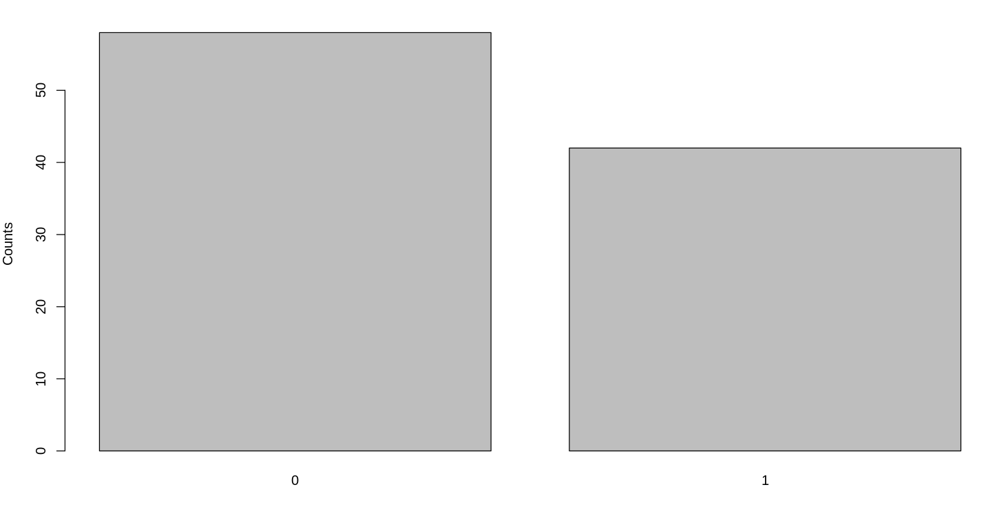
qsimulatR displays summary of the measurement and its corresponding histogram.
> meas <- measure(e1 = psi, bit = 1, repetitions = 100)
> summary(meas)
Bit 1 has been measured 100 times with the outcome:
0:  58
1:  42
>hist(meas)
The Bloch sphere
We introduce the Bloc sphere to help you understand the geometric interpretation of the H, X, Y, Z, S and T gates (unitary operations on qubits) explained later in this article.
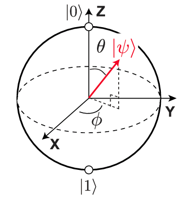
We can write any normalized (pure) quantum state as
$$|\psi> = \cos(\frac{\theta}{2})|0> + e^{i\phi} \sin(\frac{\theta}{2})|1>$$
where the angle θ ε [0, 2π] determines the probability to measure |0> or |1> states, and the angle φ ε [0, π] describes the relative phase.
All normalized (pure) states can be illustrated on the surface of a sphere with radius r, where |r| = 1. We call this sphere the Bloch sphere.
IMPORTANT*: Please be aware that the angles used in the Bloch sphere are twice as big as in the Hilbert space. Example: in the Hilbert space,* z-axis basis states |0> and |1> are orthogonal e.g. the angle is π/2=90°, but in the Bloch sphere the angle between states |0> and |1> is π \= 180° (z-axis).
The coordinates of such a state |ψ⟩ are given by the Bloch vector r
$$\vec{r} = \begin{pmatrix} \sin(\theta)\cos(\phi) \\ \sin(\theta)\sin(\phi) \\ \cos(\phi) \end{pmatrix}$$
The following are the coordinates of vector r for the following states on their corresponding axis on the Bloch spere:
$$z-axis, |0>:\hspace{0.5cm} \theta=0, \phi=arbitrary \hspace{0.5cm}\Rightarrow \vec{r}=\begin{pmatrix} 0\\ 0\\ 1 \end{pmatrix}$$
$$z-axis, |1>:\hspace{0.5cm} \theta=\pi, \phi= arbitrary \hspace{0.5cm}\Rightarrow\vec{r}=\begin{pmatrix} 0\\ 0\\ -1 \end{pmatrix}$$
$$x-axis, |+>:\hspace{0.5cm} \theta=\frac{\pi}{2}, \phi=0 \hspace{0.5cm}\Rightarrow\vec{r}=\begin{pmatrix} 1\\ 0\\ 0 \end{pmatrix}$$
$$x-axis, |->:\hspace{0.5cm} \theta=\frac{\pi}{2}, \phi=\pi \hspace{0.5cm}\Rightarrow\vec{r}=\begin{pmatrix} -1\\ 0\\ 0 \end{pmatrix}$$
$$y-axis, |+i>:\hspace{0.5cm} \theta=\frac{\pi}{2}, \phi=\frac{\pi}{2} \hspace{0.5cm}\Rightarrow\vec{r}=\begin{pmatrix} 0\\ 1\\ 0 \end{pmatrix}$$
$$y-axis, |-i>:\hspace{0.5cm} \theta=\frac{\pi}{2}, \phi=\frac{3\pi}{2} \hspace{0.5cm}\Rightarrow\vec{r}=\begin{pmatrix} 0\\ -1\\ 0 \end{pmatrix}$$
Projections
Remember that for a normalized quantum state |ψ⟩
$$|\psi> = \cos(\frac{\theta}{2})|0> + e^{i\phi} \sin(\frac{\theta}{2})|1>$$
the angle θ determines the probability to measure |0> or |1> states, and here is how these probabilities are computed:
$$Prob(0) = \cos²\theta, \hspace{.05cm}Prob(1)=\sin^2\theta$$
We say that the Z-measurement corresponds to the projection of |ψ⟩ onto the z-axis. A Z-measurement, also referred to as a measurement in the computational basis, is a common operation in quantum computing. It is associated with the Pauli Z gate and essentially measures a quantum state in the basis states |0⟩ and |1⟩.
The projections of |ψ⟩ onto the z-axis are written as
$$ = Prob(0) \hspace{1cm} = Prob(1)$$
Example: consider the quantum state |ψ⟩
$$|\psi> = \frac{1+2i}{3}|0> -\frac{2}{3} |1>$$
$$=Prob(0) = \Bigl|\frac{1+2i}{3} \Bigr|^2 = \frac{5}{9}\hspace{1cm}$$
$$=Prob(1) = \Bigl|-\frac{2}{3} \Bigr|^2 = \frac{4}{9}$$
<0| is pronounced as "bra 0". It refers to the row vector obtained by taking the conjugate-transpose of the column vector |0>, where (in addition to transposing the vector from a column vector to a row vector) each entry is replaced by its complex conjugate [1].
$$
# <0| is a row vector
> bra0 <- Conj(t(ket0@coefs))
bra0
     [,1] [,2]
[1,] 1+0i 0+0i
# |ψ> is a column vector
> psi <- qstate(nbits = 1, coefs = c((1+2i)/3, -2/3))
> psi@coefs
[1]  0.3333333+0.6666667i -0.6666667+0.0000000i
# <0|ψ> is a matrix product = inner product between the two vectors
> bra0 %*% psi@coefs
                     [,1]
[1,] 0.3333333+0.6666667i
# Probabilty to obtain 0 after measurement
> Mod(bra0 %*% psi@coefs)^2
          [,1]
[1,] 0.5555556

# Same thing for |1>
> ket1 <- X(1)*ket0
> bra1 <- Conj(t(ket1@coefs))
> bra1
     [,1] [,2]
[1,] 0+0i 1+0i
> bra1 %*% psi@coefs
              [,1]
[1,] -0.6666667+0i
> Mod(bra1 %*% psi@coefs)^2
          [,1]
[1,] 0.4444444
Hadamard gate
When running quantum algorithms we usually start with several quantum states initialized as |0>, and the first thing we do is to perform the superposition of each one of the initialized states. This is done with an operation called the Hadamard gate.
The Hadamard gate creates a uniform superposition of the quantum state.
Let us apply the H gate to |0>
> H(1)*qstate(1)
   ( 0.7071068 )    * |0>
 + ( 0.7071068 )    * |1>
Notice that coefficients values are equal to 1/sqrt(2), we can generalize this to 1/sqrt(N) where N is the number of possible states which is N=2^nbits.
So far, we have only considered nbits=1 cases since we're working with single systems taking values from the set {0, 1} of possible classical states, thus the size of the set is N = 2^1 = 2.
Notice that the Hadamard operation is reversible e.g. if we apply H(1) twice we "come back" to |0>
# Parentheses are important !!
> H(1)*( H(1)*qstate(1) )
 ( 1 )    * |0>
Let us look at the structure of the H(1) operation
> str(H(1))
Formal class 'sqgate' [package "qsimulatR"] with 3 slots
  ..@ bit : int 1
  ..@ M   : cplx [1:2, 1:2] 0.707+0i 0.707+0i 0.707+0i ...
  ..@ type: chr "H"
Notice that the M slot is a complex matrix
> H(1)@M
             [,1]          [,2]
[1,] 0.7071068+0i  0.7071068+0i
[2,] 0.7071068+0i -0.7071068+0i
We say that the H(1) operation is represented by the unitary matrix M.
$$H = \frac{1}{\sqrt{2}} \begin{pmatrix} 1 & 1 \\ -1 & 1 \\ \end{pmatrix}$$
If you multiply M by its conjugate transpose you will obtain the identity matrix.
# Conj(t(H(1)@M)): conjugate transpose of M
# e.g., transpose M and take the complex conjugate of each entry
> H(1)@M %*% Conj(t(H(1)@M))
     [,1] [,2]
[1,] 1+0i 0+0i
[2,] 0+0i 1+0i
Generally speaking, all allowable operations on quantum state vectors are presented by unitary matrices. Unitary matrices are a set of linear mappings which transform quantum state vectors to other quantum state vectors.
Here is the action of the Hadamard operation on a few qubit state vectors [1].
$$H |0> = |+>\hspace{0.5cm} H |1> = |->\hspace{0.5cm} H |+> = |0>\hspace{0.5cm} H |-> = |1>$$
# H|0>
> H(1)*qstate(1)
   ( 0.7071068 )    * |0>
 + ( 0.7071068 )    * |1>
# H|1>
> H(1)*(X(1)*qstate(1))
   ( 0.7071068 )    * |0>
 + ( -0.7071068 )    * |1>
# H|+> = HH|0> = |0>
> H(1)*(H(1)*qstate(1))
   ( 1 )    * |0>
# H|-> = HH|1> = |1>
H gate representation
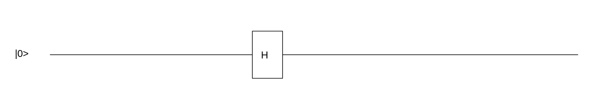
In the quantum circuit model, wires represent qubits and gates represent operations acting on these qubits. We will discuss quantum circuits in this series but for now, let us present the plot function
> x <- qstate(1)
> x <- H(1)*x # H.|0>
> qsimulatR::plot(x, qubitnames="|0>")
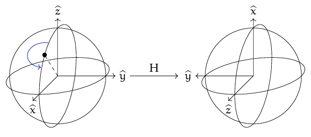
Geometric interpretation of H
In terms of the Bloch sphere, the Hadamard gate interchanges the x- and z-axis, and inverts the y-axis [5].
The GIF images included in this article come from the Learning Quantum website [6].
Let us remind ourselves of the result of applying H(1) to |0>
> H(1)*qstate(1)
   ( 0.7071068 )    * |0>
 + ( -0.7071068 )    * |1>
The result of this uniform superposition of |0> with the H gate can be labeled as "|+>" (the plus state) quantum state vector.
We say that the H(1) operation is used to exchange between the z-axis basis ({|0>, |1>}) and the x-axis basis {|+>, |->} in the Bloch sphere.
Pauli X gate - Bit Flip
Concerning the computational basis, the X gate is equivalent to a classical NOT operation, or logical negation.
The computation basis states are interchanged, so that |0⟩ becomes |1⟩ and |1⟩ becomes |0⟩.
Note: the X-gate is not a true quantum NOT gate, since it only logically negates the state in the computational basis.
Let us remind ourselves how we obtained |1> by performing a bit flip on |0>
# X.|0>
> X(1)*qstate(1)
 ( 1 )    * |1>

# X is also reversible: we come back to |0>
> X(1)*(X(1)*qstate(1))
 ( 1 )    * |0>

# Let us look at the structure of X(1)
> str(X(1))
Formal class 'sqgate' [package "qsimulatR"] with 3 slots
  ..@ bit : int 1
  ..@ M   : cplx [1:2, 1:2] 0+0i 1+0i 1+0i ...
  ..@ type: chr "X"

# We notice the Pauli matrix in the M slot
> X(1)@M
     [,1] [,2]
[1,] 0+0i 1+0i
[2,] 1+0i 0+0i

# The matrix above is a unitary matrix
> X(1)@M %*% Conj(t(X(1)@M))
     [,1] [,2]
[1,] 1+0i 0+0i
[2,] 0+0i 1+0i
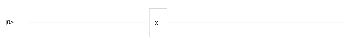
X gate representation
In the quantum circuit model, wires represent qubits and gates represent operations acting on these qubits. We will discuss quantum circuits in this series but for now, let us present the plot function
> qsimulatR::plot(X(1)*qstate(1), qubitnames="|0>")
Geometric interpretation of X
The X gate generates a half-turn in the Bloch sphere about the x-axis [5]. We say that for the X gate only the angle (θ, theta) matters, the phase (φ, phi) is arbitrary.
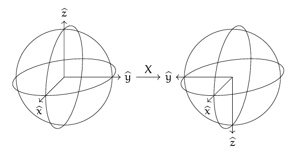
The GIF images included in this article come from the Learning Quantum website [6].
Pauli Z gate - Phase Flip
Let us perform a phase flip on the |0> and the |1> states respectively.
# Z.|0>
> Z(1)*qstate(1)
 ( 1 )    * |0>

# Z.|1>
> Z(1)*(X(1)*qstate(1))
 ( -1 )    * |1>

# Let us look at the structure of Z(1)
> str(Z(1))
Formal class 'sqgate' [package "qsimulatR"] with 3 slots
  ..@ bit : int 1
  ..@ M   : cplx [1:2, 1:2] 1+0i 0+0i 0+0i ...
  ..@ type: chr "Z"

# We notice the Pauli matrix in the M slot
> Z(1)@M
     [,1]  [,2]
[1,] 1+0i  0+0i
[2,] 0+0i -1+0i

# The matrix above is a unitary matrix
> Z(1)@M %*% Conj(t(Z(1)@M))
     [,1] [,2]
[1,] 1+0i 0+0i
[2,] 0+0i 1+0i
Thus, applying the Z gate to an initialized qubit (|0>) will leave the qubits computational state unchanged when measured. For the |1> state, notice that the complex amplitude of the resulting state is displayed as "( -1 )".
Remember, that |0> and |1> are orthogonal in the Hilbert space. Thus, concerning the computational basis, the Z gate flips the phase of the |1⟩ state relative to the |0⟩ state.
Z gate representation
In the quantum circuit model, wires represent qubits and gates represent operations acting on these qubits. We will discuss quantum circuits in this series but for now, let us present the plot function
Geometric interpretation of Z
The Pauli Z gate generates a half-turn in the Bloch sphere about the z-axis.
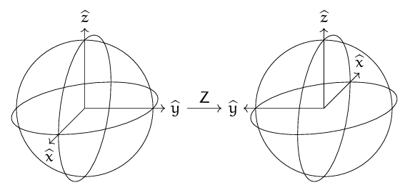
The GIF images included in this article come from the Learning Quantum website [6].
Specifically, it maps 1 to -1 and leaves 0 unchanged. It does this by rotating around the Z axis of the qubit by π radians (180 degrees). By doing this it flips the phase of the qubit.
Pauli Y gate - Bit & Phase Flip
Let us perform a bit and phase flip on the |0> state and the |1> state respectively.
# Y.|0>
> Y(1)*qstate(1)
 ( 0-1i )    * |1>

# Y.|1>
> Y(1)*(X(1)*qstate(1))
 ( 0+1i )    * |0>

# Let us look at the structure of Y(1)
> str(Y(1))
Formal class 'sqgate' [package "qsimulatR"] with 3 slots
  ..@ bit : int 1
  ..@ M   : cplx [1:2, 1:2] 0+0i 0-1i 0+1i ...
  ..@ type: chr "Y"

# We notice the Pauli matrix in the M slot
> Y(1)@M
     [,1] [,2]
[1,] 0+0i 0+1i
[2,] 0-1i 0+0i

# The matrix above is a unitary matrix
> Y(1)@M %*% Conj(t(Y(1)@M))
     [,1] [,2]
[1,] 1+0i 0+0i
[2,] 0+0i 1+0i
Concerning the computational basis, we interchange the |0> and |1> states and apply a relative phase flip.
The Y gate can be thought of as a combination of X and Z gates, Y = −iZX.
Y gate representation
In the quantum circuit model, wires represent qubits and gates represent operations acting on these qubits. We will discuss quantum circuits in this series but for now, let us present the plot function
Geometric interpretation of Y
The Pauli Y gate generates a half-turn in the Bloch sphere about the y-axis [5].
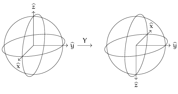
The GIF images included in this article come from the Learning Quantum website [6].
S gate - Phase gate Z90
Historically called the phase gate (and denoted by "P"), since it shifts the phase of the one state relative to the zero state [5].
Let us apply the S gate to the |0> and |1> states respectively.
# S.|0>
> S(1)*qstate(1)
 ( 1 )    * |0>

# S.|1>
> S(1)*(X(1)*qstate(1))
 ( 0+1i )    * |1>

# Let us look at the structure of S(1)
> str(S(1))
Formal class 'sqgate' [package "qsimulatR"] with 3 slots
  ..@ bit : int 1
  ..@ M   : cplx [1:2, 1:2] 1+0i 0+0i 0+0i ...
  ..@ type: chr "S"

# We notice the Pauli matrix in the M slot
> S(1)@M
     [,1] [,2]
[1,] 1+0i 0+0i
[2,] 0+0i 0+1i


# The matrix above is a unitary matrix
> S(1)@M %*% Conj(t(S(1)@M))
     [,1] [,2]
[1,] 1+0i 0+0i
[2,] 0+0i 1+0i
Note: S.H is applied to change from Z to Y basis
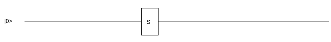
S gate representation
In the quantum circuit model, wires represent qubits and gates represent operations acting on these qubits. We will discuss quantum circuits in this series but for now, let us present the plot function
> qsimulatR::plot(S(1)*qstate(1), qubitnames="|0>")
Geometric interpretation of S
The S gate adds 90° rotation to the phase. It performs a half of the Z gate e.g., it is the square root of the Z-gate, SS = Z [5].
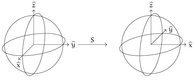
The GIF images included in this article come from the Learning Quantum website [6].
T gate - Phase gate
It performs a quarter of the Z gate and a half of the S gate.
Let us apply the S gate to the |0> and |1> states respectively.
#
T gate representation
In the quantum circuit model, wires represent qubits and gates represent operations acting on these qubits. We will discuss quantum circuits in this series but for now, let us present the plot function
Geometric interpretation of T
An eight-turn anti-clockwise about the z-axis [5].
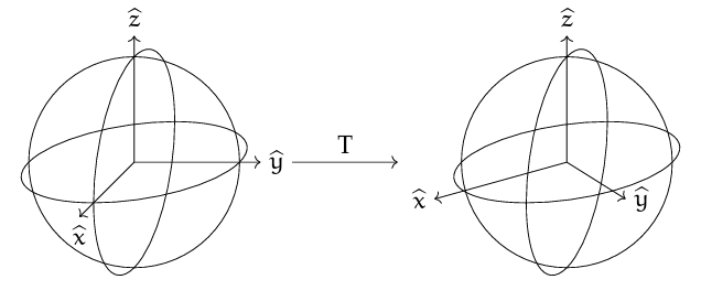
The GIF images included in this article come from the Learning Quantum website [6].

Conclusion
xx
References
[1] Ostmeyer J., Urbach C., qsimulatR: A Quantum Computer Simulator, https://cran.r-project.org/web/packages/qsimulatR/
[2] qsimulatR package vignette, https://cran.r-project.org/web/packages/qsimulatR/vignettes/qsimulatR.html
[3] Qiskit, Basics of Quantum Information, https://learn.qiskit.org/course/basics/single-systems
[4] Qiskit, Summer School 2021, https://learn.qiskit.org/summer-school/2021/lec1-1-vector-spaces-tensor-products-qubits
[5] Crooks G. E., "Gates, States, and Circuits", Tech. Note 014v0.9.0 beta, 2023-03-01
[6] Learning Quantum, Single Qubit Gates, https://lewisla.gitbook.io/learning-quantum/quantum-circuits/single-qubit-gates