


Table of contents
- Introduction
- Packages
- Hyperparameter Tuning end-to-end process
- Reminder of Part 3 results
- Cross-validation plan
- Setup parallel processing
- Prophet Boost
- Prophet Boost summary results
- Random Forest summary results
- XGBoost summary results
- Prophet summary results
- Modeltime & Calibration tables
- Model evaluation results
- Forecast plot
- Save your work
- Conclusion
- References
Cover photo by christian buehner on Unsplash
Go to R-bloggers for R news and tutorials contributed by hundreds of R bloggers.
Introduction
This is the fourth of a series of 6 articles about time series forecasting with panel data and ensemble stacking with R.
Through these articles I will be putting into practice what I have learned from the Business Science University training course 1 "DS4B 203-R: High-Performance Time Series Forecasting", delivered by Matt Dancho. If you are looking to gain a high level of expertise in time series with R I strongly recommend this course.
The objective of this article is to explain the end-to-end process of time series hyperparamter tuning for non-sequential machine learning models like Random Forest, XGBoost, Prophet, and Prophet Boost. k-fold cross-validation can be applied to non-sequential algorithms.
You will understand how to tune parameters for Prophet Boost by performing several tuning rounds to adjust and stabilize the performance of the model. The hyperparameter tuning process is the same for the other algorithms.
The provided code is highly redundant for the sake of clarity. There is a lot of room for optimization with custom functions.
Prerequisites
I assume you are already familiar with the following topics, packages and terms:
dplyr or tidyverse R packages
preprocessing recipes from Part 2
model specification and workflows from Part 3
k-fold cross-validation
parameters of Random Forest, XGBoost, Prophet, and Prophet Boost algorithms
grid search
model evaluation metrics: RMSE, R-squared, ...
Packages
The following packages must be loaded:
# 01 FEATURE ENGINEERING
library(tidyverse)  # loading dplyr, tibble, ggplot2, .. dependencies
library(timetk)  # using timetk plotting, diagnostics and augment operations
library(tsibble)  # for month to Date conversion
library(tsibbledata)  # for aus_retail dataset
library(fastDummies)  # for dummyfying categorical variables
library(skimr) # for quick statistics

# 02 FEATURE ENGINEERING WITH RECIPES
library(tidymodels) # with workflow dependency

# 03 MACHINE LEARNING
library(modeltime) # ML models specifications and engines
library(tictoc) # measure training elapsed time

# 04 HYPERPARAMETER TUNING
library(future)
library(doFuture)
library(plotly)
Hyperparameter Tuning end-to-end process
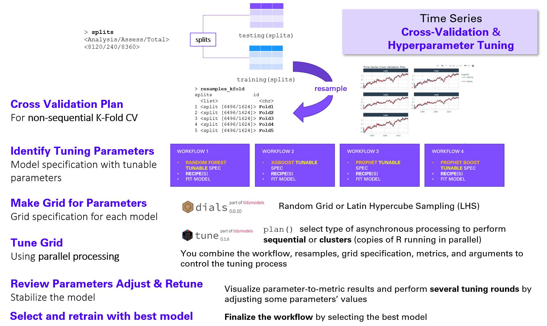
The end-to-end process is as follows:
Get the resamples. Here we will perform a k-fold cross-validation and obtain a cross-validation plan that we can plot to see "inside the folds".
Prepare for parallel process: register to future and get the number of vCores.
Define the tunable model specification: explicitly indicate the tunable parameters.
Define a tunable workflow into which we add the tunable model specification and the existing recipe; update the recipe if necessary.
Verify that the system has all tunable parameters' range, some parameter such as
mtrydo not have its values range correctly initialized.Define the search grid specification: you must provide type of grid (random or latin hypercube sampling) and its size.
Toggle on the parallel processing
Run the hyperparameter tuning by provding the tunable workflow, the resamples, and the grid specification.
Run several tuning rounds if you can e.g., if you have the time and resources and/or you are able to fix some parameter ranges.
After several tuning rounds, select the best model: with the lowest RMSE or with the higest R-squared, it may be same model or they can be different models.
(Re)fit the best model(s) with the training data by providing the tuned workflow.
Reminder of Part 3 results
Let us recall the non-tuned model evaluation results for the 4 machine learning algorithms:
# Load saved work from Part 3
> wflw_artifacts <- read_rds("workflows_artifacts_list.rds")

> wflw_artifacts$calibration$calibration_tbl %>%
   modeltime_accuracy(testing(splits)) %>%
   arrange(rmse)

# A tibble: 4 x 9
  .model_id .model_desc               .type   mae  mape  mase smape  rmse   rsq
      <int> <chr>                     <chr> <dbl> <dbl> <dbl> <dbl> <dbl> <dbl>
1         3 PROPHET W/ REGRESSORS     Test  0.213  22.9 0.470  22.9 0.267 0.846
2         4 PROPHET W/ XGBOOST ERRORS Test  0.203  27.1 0.448  20.6 0.283 0.750
3         2 XGBOOST                   Test  0.228  26.9 0.503  22.7 0.306 0.761
4         1 RANGER                    Test  0.244  25.6 0.538  25.3 0.322 0.763
Note: "RANGER" is the default engine for Random Forest modeltime::rand_forest().
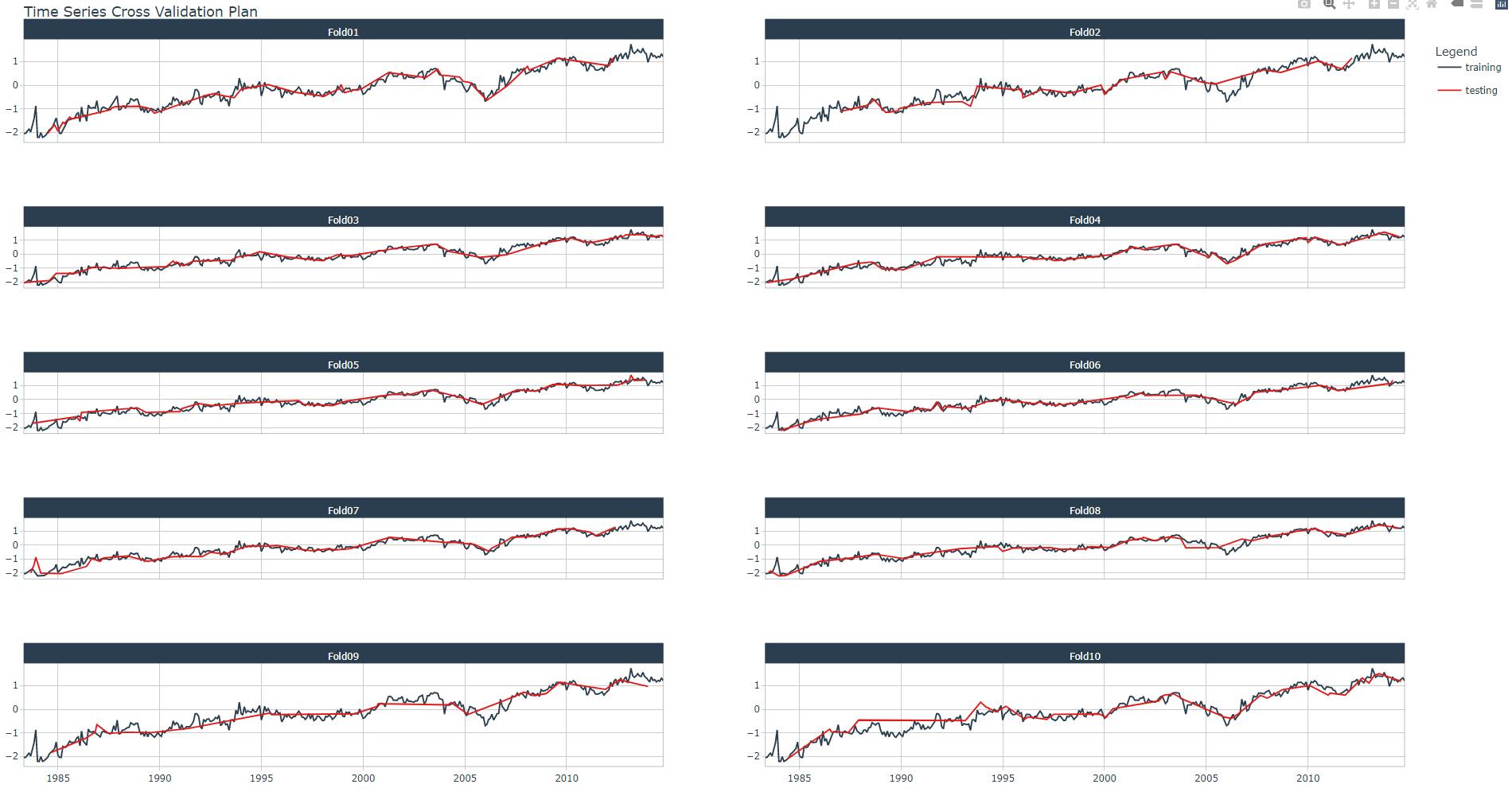
Cross-validation plan
A k-fold cross-validation will randomly split the training data into k groups of roughly equal size (called "folds"). A resample of the analysis data consisted of k-1 of the folds while the assessment set contains the final fold. In basic k-fold cross-validation (i.e. no repeats), the number of resamples is equal to k.
It is important to understand that you may perform a k-fold cross-validation for all four machine learning models since they are non-sequential models. This is not the case for other models such as ARIMA, ETS (exponential smoothing) and NNETAR for which you should perform a time_series_cv() cross-validation.
Perform the resample with function rsample::vfold_cv() as shown in the code snippet below. You may also display the cross validation plan and its plot (here, for one Industry) with tk_time_series_cv_plan() and plot_time_series_cv_plan(), respectively.
# k = 10 folds
> set.seed(123)
> resamples_kfold <- training(splits) %>%
  vfold_cv(v = 10)

resamples_kfold %>%
  tk_time_series_cv_plan() %>%
  filter(Industry == Industries[1]) %>%
  plot_time_series_cv_plan(.date_var = Month,
                             .value = Turnover,
                             .facet_ncol = 2)
Setup parallel processing
As per 1, "the future library allows for evaluating R expressions asynchronously. The doFuture package is an adapter that provides for running loops in parallel. The tune package manages the adapter process internally, so all we need to do is to set up doFuture".
# Registers the doFuture parallel processing
registerDoFuture()

# My laptop i5-8350U CPU has 8 threads (or vCores)
n_cores <- parallel::detectCores()
Prophet Boost
Prophet Boost - Identify tuning parameters
I've decided to tune the following parameters, you can run ?prophet_boost for a full description:
changepoint_num(prophet): Number of potential changepoints to include for modeling trend.mtry(xgboost): An integer for the number of predictors that will be randomly sampled at each split when creating the tree models.trees(xgboost): An integer for the number of trees contained in the ensemblemin_n(xgboost): An integer for the minimum number of data points in a node that are required for the node to be split further. tree_depth: An integer for the maximum depth of the tree (i.e. number of splits) (specific engines only).learn_rate(xgboost): A number for the rate at which the boosting algorithm adapts from iteration-to-iteration.loss_reduction(xgboost): A number for the reduction in the loss function required to split further.tree_depth(xgboost): An integer for the maximum depth of the tree (i.e. number of splits).
Define the tunable parameters with tune() within the model specification of prophet_boost(). Then, define a new tunable workflow for Prophet Boost (wflw_spec_rf_tune) by adding the tunable specification and the same recipe as in Part 3. Display the summary of the workflow as shown in the code snippet below.
> model_spec_prophet_boost_tune <- prophet_boost(

  mode = "regression",
  # growth = NULL,
  changepoint_num = tune(),
  #changepoint_range = NULL,
  seasonality_yearly = FALSE,
  seasonality_weekly = FALSE,
  seasonality_daily = FALSE,
  # season = NULL,
  # prior_scale_changepoints = NULL,
  # prior_scale_seasonality = NULL,
  # prior_scale_holidays = NULL,
  # logistic_cap = NULL,
  # logistic_floor = NULL,
  mtry = tune(),
  trees = tune(),
  min_n = tune(),
  tree_depth = tune(),
  learn_rate = tune(),
  loss_reduction = tune(),
  # sample_size = NULL,
  # stop_iter = NULL

) %>%
  set_engine("prophet_xgboost")

> wflw_spec_prophet_boost_tune <- workflow() %>%
  add_model(model_spec_prophet_boost_tune) %>%
  add_recipe(artifacts$recipes$recipe_spec)

> wflw_spec_prophet_boost_tune
== Workflow ===================================================================================================================================
Preprocessor: Recipe
Model: prophet_boost()

-- Preprocessor -------------------------------------------------------------------------------------------------------------------------------
5 Recipe Steps

* step_other()
* step_timeseries_signature()
* step_rm()
* step_dummy()
* step_normalize()

-- Model --------------------------------------------------------------------------------------------------------------------------------------
PROPHET Regression Model Specification (regression)

Main Arguments:
  changepoint_num = tune()
  seasonality_yearly = FALSE
  seasonality_weekly = FALSE
  seasonality_daily = FALSE
  mtry = tune()
  trees = tune()
  min_n = tune()
  tree_depth = tune()
  learn_rate = tune()
  loss_reduction = tune()

Computational engine: prophet_xgboost
Prophet Boost - Grid spec
Check parameters' range
The first thing to do is to display the parameters of the model with extract_parameter_set_dials(): you must check if there is any parameter with missing information about its values range.
As shown below, nparam[?] means that values range is missing for mtry parameter.
> extract_parameter_set_dials(model_spec_prophet_boost_tune)
Collection of 3 parameters for tuning

 identifier  type    object
       mtry  mtry nparam[?]
      trees trees nparam[+]
      min_n min_n nparam[+]

Model parameters needing finalization:
   # Randomly Selected Predictors ('mtry')

See `?dials::finalize` or `?dials::update.parameters` for more information.
Check the number of predictors looking at the recipe's summary.
> artifacts$recipes$recipe_spec %>%
   update_role(Month, new_role = "indicator") %>%
   prep() %>%
   summary() %>%
   group_by(role) %>%
   summarise(n=n())
# A tibble: 3 x 2
  role          n
  <chr>     <int>
1 indicator     1
2 outcome       1
3 predictor    50
The new range update will be applied within the grid specifications in the next code snippet.
Grid search specification
Thanks to the dials package it is possible to define specifications for either Random Grid or Latin Hypercube Sampling (LHS).
We define a grid of size 20 e.g. 20 random values combinations of the 7 tunable parameters. Remember to set the seed to fix the grid since it uses a random process, you may have different values.
Since we have defined a 10-fold cross-validation there will be 20 predictions per fold and the mean of the performance metric (RMSE, R-squared, ...) will be calculated.
set.seed(123)
grid_spec_1 <- grid_latin_hypercube(
  extract_parameter_set_dials(model_spec_prophet_boost_tune) %>%
    update(mtry = mtry(range = c(1, 50))),
  size = 20
)

> grid_spec_1
# A tibble: 20 x 7
   changepoint_num  mtry trees min_n tree_depth learn_rate loss_reduction
             <int> <int> <int> <int>      <int>      <dbl>          <dbl>
 1               6     9   145    26          5   2.50e- 7       1.89e- 6
 2              33    33  1538    18         14   5.55e- 6       2.17e- 2
 3               8    42    42    21          3   2.22e- 6       1.63e- 1
 4               0    23  1183     4         12   2.44e- 3       1.91e-10
 5              30    30  1261    25         11   1.34e- 9       1.90e- 8
 6              22     5  1882     3          7   1.45e- 8       1.01e- 7
 7              45    48   971    30          6   2.94e-10       5.34e- 3
 8              20     7   798    27         15   1.18e- 4       4.65e- 9
 9              14    22  1993    12          3   6.54e- 7       1.42e- 4
10              27    37  1620    35          8   3.16e- 2       7.35e- 8
11              23    45  1450     8          4   6.11e- 4       7.60e- 2
12              31     1  1756    14         13   8.92e- 8       2.41e- 3
13              37    19   402    39          9   2.28e- 9       4.83e- 4
14              39    46   245    31         11   2.60e- 8       9.67e- 7
15              42    13   336    37          2   6.48e- 3       5.83e-10
16              17    28  1311    34          8   2.41e-10       2.92e- 5
17              49    31   870    11          2   2.32e- 5       1.70e+ 1
18               4    13   575     8         13   2.68e- 4       1.09e+ 0
19              44    18  1097    20         10   3.33e- 5       5.98e+ 0
20              11    40   613    16          6   5.62e- 2       7.32e- 6
Prophet Boost - Tune Grid
Let us perform 3 tuning rounds with 3 different grid specifications. I will explain at each round why do we perform the corresponding grid spec:
Round 1 with
grid_spec_1Round 2 with
grid_spec_2Round 3 with
grid_spec_3
To tune the workflow with a grid you need to provide the resamples, the grid specification and some controls on the grid search process.
tic()
tune_results_prophet_boost_1 <- wflw_spec_prophet_boost_tune %>%
  tune_grid(
    resamples  = resamples_kfold,
    grid = grid_spec_1,
    control = control_grid(verbose = TRUE,
                           allow_par = TRUE)
  )
toc()

> plan(strategy = sequential)

> tune_results_prophet_boost_1 %>%
+     show_best("rmse", n = Inf)
# A tibble: 20 x 13
   changepoint_num  mtry trees min_n tree_depth learn_rate loss_reduction .metric .estimator  mean     n std_err .config
             <int> <int> <int> <int>      <int>      <dbl>          <dbl> <chr>   <chr>      <dbl> <int>   <dbl> <chr>
 1              11    40   613    16          6   5.62e- 2       7.32e- 6 rmse    standard   0.185    10 0.00372 Preprocessor~
 2              27    37  1620    35          8   3.16e- 2       7.35e- 8 rmse    standard   0.187    10 0.00378 Preprocessor~
 3               0    23  1183     4         12   2.44e- 3       1.91e-10 rmse    standard   0.192    10 0.00422 Preprocessor~
 4              42    13   336    37          2   6.48e- 3       5.83e-10 rmse    standard   0.308    10 0.00407 Preprocessor~
 5              23    45  1450     8          4   6.11e- 4       7.60e- 2 rmse    standard   0.360    10 0.00406 Preprocessor~
 6               4    13   575     8         13   2.68e- 4       1.09e+ 0 rmse    standard   0.550    10 0.00560 Preprocessor~
 7              20     7   798    27         15   1.18e- 4       4.65e- 9 rmse    standard   0.579    10 0.00588 Preprocessor~
 8              44    18  1097    20         10   3.33e- 5       5.98e+ 0 rmse    standard   0.606    10 0.00605 Preprocessor~
 9              49    31   870    11          2   2.32e- 5       1.70e+ 1 rmse    standard   0.614    10 0.00619 Preprocessor~
10              33    33  1538    18         14   5.55e- 6       2.17e- 2 rmse    standard   0.619    10 0.00617 Preprocessor~
11              14    22  1993    12          3   6.54e- 7       1.42e- 4 rmse    standard   0.623    10 0.00619 Preprocessor~
12              17    28  1311    34          8   2.41e-10       2.92e- 5 rmse    standard   0.623    10 0.00620 Preprocessor~
13              39    46   245    31         11   2.60e- 8       9.67e- 7 rmse    standard   0.623    10 0.00620 Preprocessor~
14              31     1  1756    14         13   8.92e- 8       2.41e- 3 rmse    standard   0.623    10 0.00621 Preprocessor~
15              22     5  1882     3          7   1.45e- 8       1.01e- 7 rmse    standard   0.623    10 0.00621 Preprocessor~
16              37    19   402    39          9   2.28e- 9       4.83e- 4 rmse    standard   0.623    10 0.00620 Preprocessor~
17               8    42    42    21          3   2.22e- 6       1.63e- 1 rmse    standard   0.623    10 0.00617 Preprocessor~
18              45    48   971    30          6   2.94e-10       5.34e- 3 rmse    standard   0.623    10 0.00619 Preprocessor~
19              30    30  1261    25         11   1.34e- 9       1.90e- 8 rmse    standard   0.623    10 0.00619 Preprocessor~
20               6     9   145    26          5   2.50e- 7       1.89e- 6 rmse    standard   0.624    10 0.00616 Preprocessor~

> tune_results_prophet_boost_1 %>%
+     show_best("rsq", n = Inf)
# A tibble: 20 x 13
   changepoint_num  mtry trees min_n tree_depth learn_rate loss_reduction .metric .estimator  mean     n std_err .config
             <int> <int> <int> <int>      <int>      <dbl>          <dbl> <chr>   <chr>      <dbl> <int>   <dbl> <chr>
 1              11    40   613    16          6   5.62e- 2       7.32e- 6 rsq     standard   0.958    10 0.00191 Preprocessor~
 2              27    37  1620    35          8   3.16e- 2       7.35e- 8 rsq     standard   0.957    10 0.00195 Preprocessor~
 3               0    23  1183     4         12   2.44e- 3       1.91e-10 rsq     standard   0.956    10 0.00218 Preprocessor~
 4              23    45  1450     8          4   6.11e- 4       7.60e- 2 rsq     standard   0.893    10 0.00325 Preprocessor~
 5              42    13   336    37          2   6.48e- 3       5.83e-10 rsq     standard   0.888    10 0.00293 Preprocessor~
 6               4    13   575     8         13   2.68e- 4       1.09e+ 0 rsq     standard   0.855    10 0.00460 Preprocessor~
 7              20     7   798    27         15   1.18e- 4       4.65e- 9 rsq     standard   0.845    10 0.00511 Preprocessor~
 8              44    18  1097    20         10   3.33e- 5       5.98e+ 0 rsq     standard   0.835    10 0.00535 Preprocessor~
 9              33    33  1538    18         14   5.55e- 6       2.17e- 2 rsq     standard   0.832    10 0.00551 Preprocessor~
10              49    31   870    11          2   2.32e- 5       1.70e+ 1 rsq     standard   0.832    10 0.00549 Preprocessor~
11              14    22  1993    12          3   6.54e- 7       1.42e- 4 rsq     standard   0.830    10 0.00555 Preprocessor~
12              17    28  1311    34          8   2.41e-10       2.92e- 5 rsq     standard   0.830    10 0.00557 Preprocessor~
13              39    46   245    31         11   2.60e- 8       9.67e- 7 rsq     standard   0.830    10 0.00557 Preprocessor~
14              22     5  1882     3          7   1.45e- 8       1.01e- 7 rsq     standard   0.830    10 0.00557 Preprocessor~
15              45    48   971    30          6   2.94e-10       5.34e- 3 rsq     standard   0.830    10 0.00556 Preprocessor~
16              37    19   402    39          9   2.28e- 9       4.83e- 4 rsq     standard   0.830    10 0.00558 Preprocessor~
17               8    42    42    21          3   2.22e- 6       1.63e- 1 rsq     standard   0.830    10 0.00554 Preprocessor~
18              30    30  1261    25         11   1.34e- 9       1.90e- 8 rsq     standard   0.830    10 0.00557 Preprocessor~
19              31     1  1756    14         13   8.92e- 8       2.41e- 3 rsq     standard   0.830    10 0.00557 Preprocessor~
20               6     9   145    26          5   2.50e- 7       1.89e- 6 rsq     standard   0.829    10 0.00552 Preprocessor~
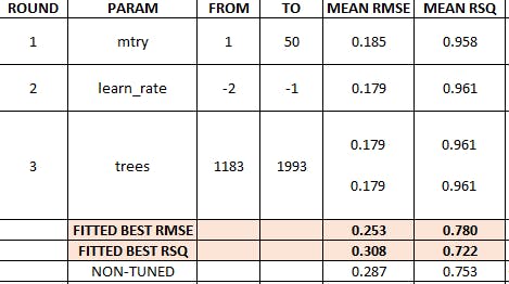
Round 1
Plot the tuning results for analysis. You may pipe the tuning results into feasts::autoplot() and generated and plot an interactive ggplot object with ggplotly, as shown in the code snippet below:
gr1<- tune_results_prophet_boost %>%
  autoplot() +
  geom_smooth(se = FALSE)

ggplotly(gr1)
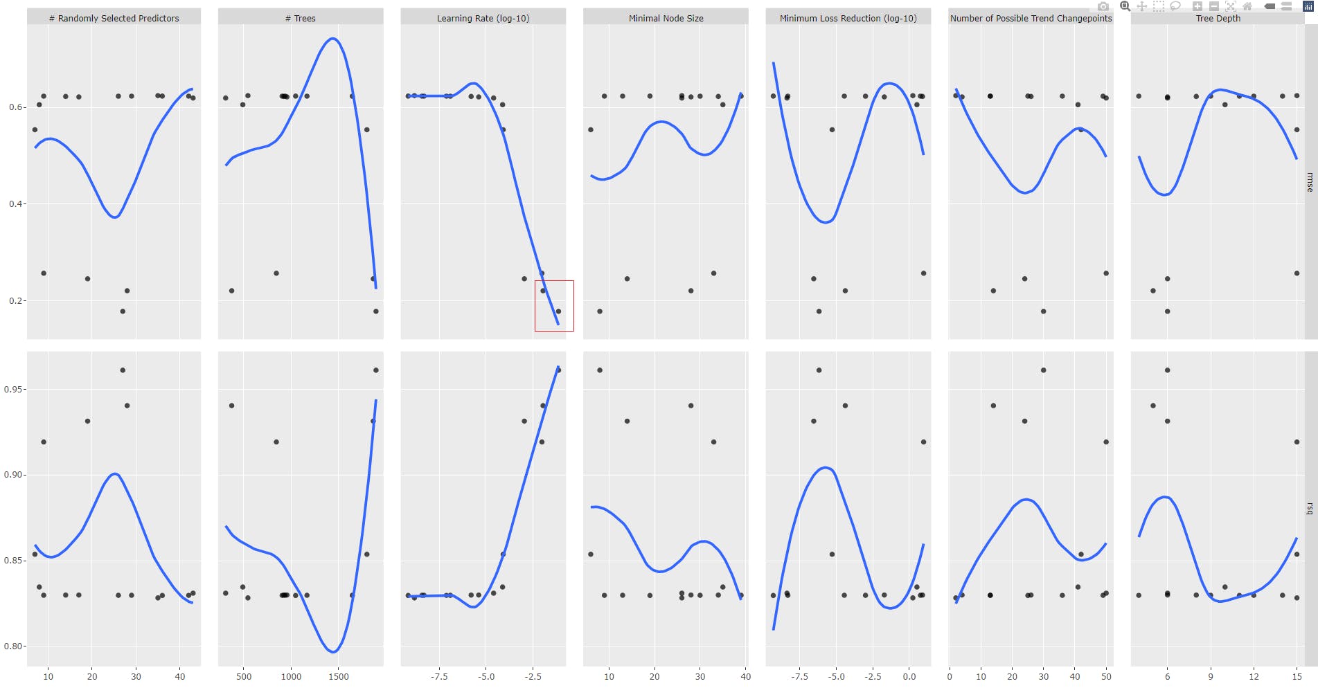
This is the most important part of the process: as a data scientist, you will decide of the tuning strategy.
Try to spot the plot with a monotonic smooth fonction (blue line), descending for RMSE or ascending for R-squared. Here, it corresponds to "Learning Rate (log-10)" parameter. Update the grid spec with a new range of values for Learning Rate where the RMSE is minimal.
Generally speaking we will do the following steps for each tuning round
update or adjust the parameter range within the grid specification.
toggle on parallel processing
perform hyperparameter tuning with new grid specification
toggle off parallel processing
analyze best RMSE and RSQ results
go to 1.
Round 2
We fix learn_rate parameter range of values.
# 1. update or adjust the parameter range within the grid specification.
set.seed(123)
grid_spec_2 <- grid_latin_hypercube(
  extract_parameter_set_dials(model_spec_prophet_boost_tune) %>%
    update(mtry = mtry(range = c(1, 50)),
           learn_rate = learn_rate(range = c(-2.0, -1.0))),
  size = 20
)

# 2. toggle on parallel processing
plan(
  strategy = cluster,
  workers  = parallel::makeCluster(n_cores)
)

# 3. perform hyperparameter tuning with new grid specification
tic()
tune_results_prophet_boost_2 <- wflw_spec_prophet_boost_tune %>%
  tune_grid(
    resamples  = resamples_kfold,
    grid = grid_spec_2,
    control = control_grid(verbose = TRUE,
                           allow_par = TRUE)
  )
toc()

# 4. toggle off parallel processing
plan(strategy = sequential)

# 5. analyze best RMSE and RSQ results (here top 2)
> tune_results_prophet_boost_2 %>%
+     show_best("rsq", n = 2)
# A tibble: 2 x 13
  changepoint_num  mtry trees min_n tree_depth learn_rate loss_reduction .metric .estimator  mean     n std_err .config
            <int> <int> <int> <int>      <int>      <dbl>          <dbl> <chr>   <chr>      <dbl> <int>   <dbl> <chr>
1               0    23  1183     4         12     0.0662       1.91e-10 rsq     standard   0.961    10 0.00217 Preprocessor1~
2              11    40   613    16          6     0.0938       7.32e- 6 rsq     standard   0.960    10 0.00171 Preprocessor1~

> tune_results_prophet_boost_2 %>%
+     show_best("rmse", n = 2)
# A tibble: 2 x 13
  changepoint_num  mtry trees min_n tree_depth learn_rate loss_reduction .metric .estimator  mean     n std_err .config
            <int> <int> <int> <int>      <int>      <dbl>          <dbl> <chr>   <chr>      <dbl> <int>   <dbl> <chr>
1               0    23  1183     4         12     0.0662       1.91e-10 rmse    standard   0.179    10 0.00462 Preprocessor1~
2              11    40   613    16          6     0.0938       7.32e- 6 rmse    standard   0.181    10 0.00340 Preprocessor1~
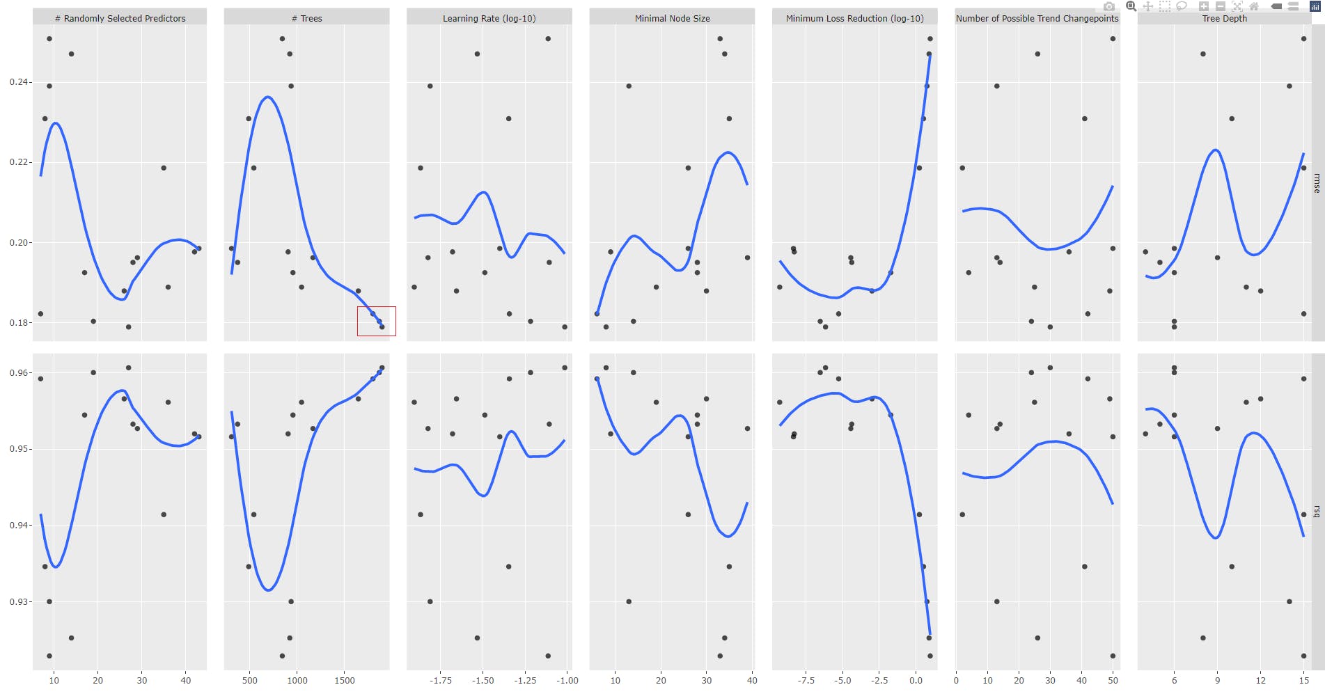
Let us analyse the plot
gr2 <- tune_results_prophet_boost_2 %>%
  autoplot() +
  geom_smooth(se = FALSE)

ggplotly(gr2)
Round 3
We fix trees parameter range of values.
set.seed(123)
grid_spec_3 <- grid_latin_hypercube(
  extract_parameter_set_dials(model_spec_prophet_boost_tune) %>%
    update(mtry = mtry(range = c(1, 50)),
           learn_rate = learn_rate(range = c(-2.0, -1.0)),
           trees = trees(range = c(1183, 1993))),
  size = 20
)

plan(
  strategy = cluster,
  workers  = parallel::makeCluster(n_cores)
)

tic()
tune_results_prophet_boost_3 <- wflw_spec_prophet_boost_tune %>%
  tune_grid(
    resamples  = resamples_kfold,
    grid = grid_spec_3,
    control = control_grid(verbose = TRUE,
                           allow_par = TRUE)
  )
toc()

plan(strategy = sequential)

> tune_results_prophet_boost_3 %>%
+     show_best("rmse", n = 2)
# A tibble: 2 x 13
  changepoint_num  mtry trees min_n tree_depth learn_rate loss_reduction .metric .estimator  mean     n std_err .config
            <int> <int> <int> <int>      <int>      <dbl>          <dbl> <chr>   <chr>      <dbl> <int>   <dbl> <chr>
1               0    23  1662     4         12     0.0662       1.91e-10 rmse    standard   0.179    10 0.00464 Preprocessor1~
2              11    40  1431    16          6     0.0938       7.32e- 6 rmse    standard   0.179    10 0.00363 Preprocessor1~

> tune_results_prophet_boost_3 %>%
+     show_best("rsq", n = 2)
# A tibble: 2 x 13
  changepoint_num  mtry trees min_n tree_depth learn_rate loss_reduction .metric .estimator  mean     n std_err .config
            <int> <int> <int> <int>      <int>      <dbl>          <dbl> <chr>   <chr>      <dbl> <int>   <dbl> <chr>
1              11    40  1431    16          6     0.0938       7.32e- 6 rsq     standard   0.961    10 0.00174 Preprocessor1~
2               0    23  1662     4         12     0.0662       1.91e-10 rsq     standard   0.961    10 0.00220 Preprocessor1~
We obtain two best models, they show the same RMSE and RSQ values because there are rounded figures.
Select and fit the best model(s)
Please recall that we deal with workflows (not models directly) which incoporate a a model and a preprocessing recipe.
We finalize (finalize_workflow()) the tuning process by selecting the best model (select_best()) from round 3 tuning results (tune_results_prophet_boost_3) and finally, we refit the model (fit(training(splits))), and display accuracy results.
# Fitting round 3 best RMSE model
set.seed(123)
wflw_fit_prophet_boost_tuned <- wflw_spec_prophet_boost_tune %>%
  finalize_workflow(
    select_best(tune_results_prophet_boost_3, "rmse", n=1)) %>%
  fit(training(splits))

modeltime_table(wflw_fit_prophet_boost_tuned) %>%
  modeltime_calibrate(testing(splits)) %>%
  modeltime_accuracy()

# A tibble: 1 x 9
  .model_id .model_desc               .type   mae  mape  mase smape  rmse   rsq
      <int> <chr>                     <chr> <dbl> <dbl> <dbl> <dbl> <dbl> <dbl>
1         1 PROPHET W/ XGBOOST ERRORS Test  0.191  25.7 0.421  19.9 0.253 0.780

# Fitting round 3 best RSQmodel
set.seed(123)
wflw_fit_prophet_boost_tuned_rsq <- wflw_spec_prophet_boost_tune %>%
  finalize_workflow(
    select_best(tune_results_prophet_boost_3, "rsq", n=1)) %>%
  fit(training(splits))

modeltime_table(wflw_fit_prophet_boost_tuned_rsq) %>%
  modeltime_calibrate(testing(splits)) %>%
  modeltime_accuracy()

# A tibble: 1 x 9
  .model_id .model_desc               .type   mae  mape  mase smape  rmse   rsq
      <int> <chr>                     <chr> <dbl> <dbl> <dbl> <dbl> <dbl> <dbl>
1         1 PROPHET W/ XGBOOST ERRORS Test  0.223  26.2 0.492  22.3 0.308 0.722
As shown above, the best fitted model is the first one, thus we select and save it.
Save Prophet Boot tuning artifacts
It is very helpful the save all artifacts of the tuning process. I've created a saved to an RDS file a R list for which the structure should the same for all algorithms.
tuned_prophet_xgb <- list(

  # Workflow spec
  tune_wkflw_spec = wflw_spec_prophet_boost_tune,
  # Grid spec
  tune_grid_spec = list(
    round1 = grid_spec_1,
    round2 = grid_spec_2,
    round3 = grid_spec_3),
  # Tuning Results
  tune_results = list(
    round1 = tune_results_prophet_boost_1,
    round2 = tune_results_prophet_boost_2,
    round3 = tune_results_prophet_boost_3),
  # Tuned Workflow Fit
  tune_wflw_fit = wflw_fit_prophet_boost_tuned,
  # from FE
  splits        = artifacts$splits,
  data          = artifacts$data,
  recipes       = artifacts$recipes,
  standardize   = artifacts$standardize,
  normalize     = artifacts$normalize

)

tuned_prophet_xgb %>%
  write_rds("tuning/tuned_prophet_xgb.rds")
Prophet Boost summary results
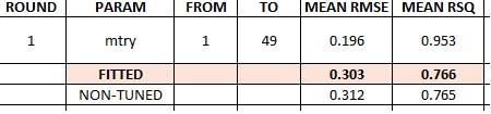
Random Forest summary results
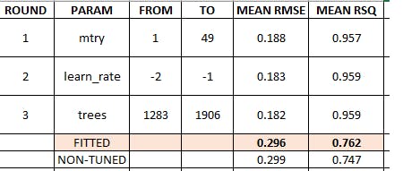
XGBoost summary results
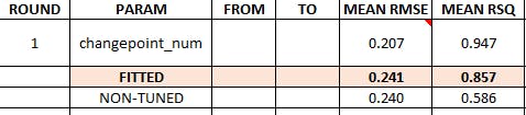
Prophet summary results
Modeltime & Calibration tables
The objective is to add all non-tuned and tuned models into a single modeltime table submodels_all_tbl.
Please recall that we deal with workflows (not models directly) which incoporates a model and a preprocessing recipe.
Notice how we combined (combine_modeltime_tables()) the tables and updated the description (update_model_description()) for the tuned workflows.
> submodels_tbl <- modeltime_table(
  wflw_artifacts$workflows$wflw_random_forest,
  wflw_artifacts$workflows$wflw_xgboost,
  wflw_artifacts$workflows$wflw_prophet,
  wflw_artifacts$workflows$wflw_prophet_boost
)

> submodels_all_tbl <- modeltime_table(
  tuned_rf_rds$tune_wflw_fit,
  tuned_xgboost_rds$tune_wflw_fit,
  tuned_prophet_rds$tune_wflw_fit,
  tuned_prophet_fou_boost_rds$tune_wflw_fit
) %>%
  update_model_description(1, "RANGER - Tuned") %>%
  update_model_description(2, "XGBOOST - Tuned") %>%
  update_model_description(3, "PROPHET W/ REGRESSORS - Tuned") %>%
  update_model_description(4, "PROPHET W/ XGBOOST ERRORS - Tuned") %>%
  combine_modeltime_tables(submodels_tbl)

> submodels_all_tbl
# Modeltime Table
# A tibble: 8 x 3
  .model_id .model     .model_desc
      <int> <list>     <chr>
1         1 <workflow> RANGER - Tuned
2         2 <workflow> XGBOOST - Tuned
3         3 <workflow> PROPHET W/ REGRESSORS - Tuned
4         4 <workflow> PROPHET W/ XGBOOST ERRORS - Tuned
5         5 <workflow> RANGER
6         6 <workflow> XGBOOST
7         7 <workflow> PROPHET W/ REGRESSORS
8         8 <workflow> PROPHET W/ XGBOOST ERRORS
Model evaluation results
We calibrate all fitted workflows with the test dataset and display the accuracy results for all non-tuned and tuned models. You may also create an interactive table which facilitates sorting, as shown in the code snippet below.
> calibration_all_tbl <- submodels_all_tbl %>%
  modeltime_calibrate(testing(splits))

calibration_all_tbl %>%
  modeltime_accuracy() %>%
  arrange(rmse)

# A tibble: 8 x 9
  .model_id .model_desc                       .type   mae  mape  mase smape  rmse   rsq
      <int> <chr>                             <chr> <dbl> <dbl> <dbl> <dbl> <dbl> <dbl>
1         7 PROPHET W/ REGRESSORS             Test  0.189  21.6 0.417  21.5 0.240 0.856
2         3 PROPHET W/ REGRESSORS - Tuned     Test  0.189  21.6 0.418  21.5 0.241 0.857
3         4 PROPHET W/ XGBOOST ERRORS - Tuned Test  0.191  25.7 0.421  19.9 0.253 0.780
4         8 PROPHET W/ XGBOOST ERRORS         Test  0.204  24.8 0.451  20.8 0.287 0.753
5         2 XGBOOST - Tuned                   Test  0.219  23.6 0.482  22.9 0.296 0.762
6         6 XGBOOST                           Test  0.216  25.0 0.476  22.4 0.299 0.747
7         1 RANGER - Tuned                    Test  0.231  26.1 0.509  24.6 0.303 0.766
8         5 RANGER                            Test  0.235  25.4 0.519  25.0 0.312 0.765

calibration_all_tbl %>%
  modeltime_accuracy() %>%
  arrange(desc(rsq))

# A tibble: 8 x 9
  .model_id .model_desc                       .type   mae  mape  mase smape  rmse   rsq
      <int> <chr>                             <chr> <dbl> <dbl> <dbl> <dbl> <dbl> <dbl>
1         3 PROPHET W/ REGRESSORS - Tuned     Test  0.189  21.6 0.418  21.5 0.241 0.857
2         7 PROPHET W/ REGRESSORS             Test  0.189  21.6 0.417  21.5 0.240 0.856
3         4 PROPHET W/ XGBOOST ERRORS - Tuned Test  0.191  25.7 0.421  19.9 0.253 0.780
4         1 RANGER - Tuned                    Test  0.231  26.1 0.509  24.6 0.303 0.766
5         5 RANGER                            Test  0.235  25.4 0.519  25.0 0.312 0.765
6         2 XGBOOST - Tuned                   Test  0.219  23.6 0.482  22.9 0.296 0.762
7         8 PROPHET W/ XGBOOST ERRORS         Test  0.204  24.8 0.451  20.8 0.287 0.753
8         6 XGBOOST                           Test  0.216  25.0 0.476  22.4 0.299 0.747

# Interactive table (bonus !)
calibration_all_tbl %>%
  modeltime_accuracy() %>%
  table_modeltime_accuracy()
Best fitted models are Prophet (best RMSE) and tuned Prophet (best RSQ).
Forecast plot
We plot a forecast with test data using all models and industries, the figure below is a zoom of the test data predictions vs. actual data.
calibration_all_tbl %>%
  modeltime_forecast(
    new_data    = testing(splits),
    actual_data = artifacts$data$data_prepared_tbl,
    keep_data   = TRUE
  ) %>%
  filter(Industry == Industries[1]) %>%
  plot_modeltime_forecast(
    #.facet_ncol         = 4,
    .conf_interval_show = FALSE,
    .interactive        = TRUE,
    .title = Industries[1]
  )
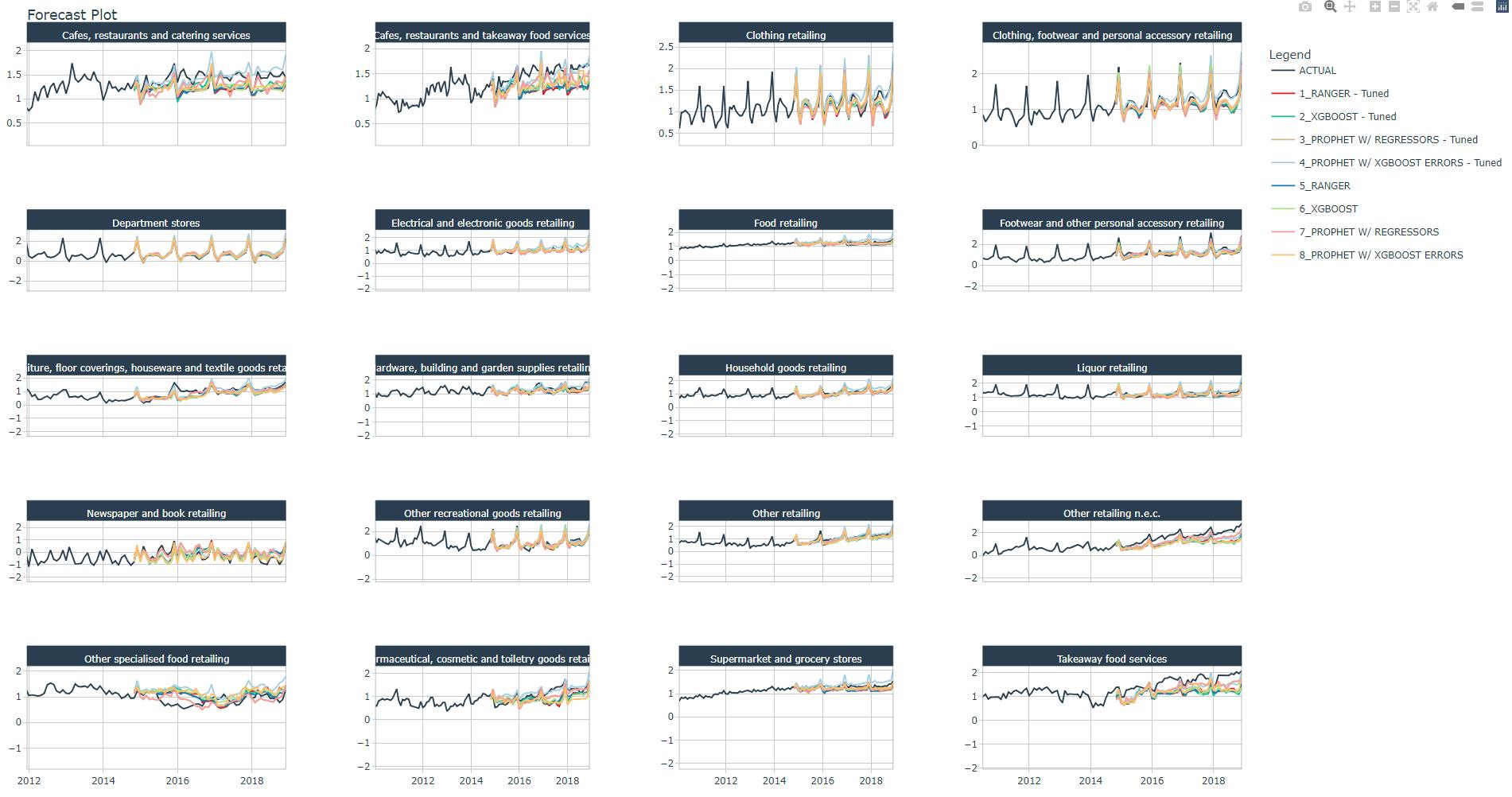
You may check and confirm the models that best follow the trend and spikes.
Save your work
workflow_all_artifacts <- list(

  workflows = submodels_all_tbl,

  calibration = calibration_all_tbl
)

workflow_all_artifacts %>%
    write_rds("workflows_NonandTuned_artifacts_list.rds")
Conclusion
In this article you have learned how to perform hyperparameter tuning for 4 machine learning (non-sequentual) models: Random Forest, XGBoost, Prophet and Prohet Boost. A step-by-step detailed process was provided for Prophet Boost.
You have learned
how to define tunable specifications for each machine learning algorithm.
how to set up parallel processing with a cluster of vCores.
how to verify parameter values range prior tuning.
how to define a grid search specification for each algorithm
how to perform hyperparameter tuning and anlyse results with the plot against RMSE.
how to adjust a specific parameter and retune, performing several hyperparameter tuning rounds.
how to select the model and retrain the model.
how to add all tuned and non-tuned models into a modeltime and calibration table.
how to display all models accuracy results and plot forecast against the test dataset.
References
1 Dancho, Matt, "DS4B 203-R: High-Performance Time Series Forecasting", Business Science University