

Cover photo by NatalyaBurova ref. 1308269282 on iStock
Go to R-bloggers for R news and tutorials contributed by hundreds of R bloggers.
This is the third article of the Quantum Computing simulation with R series.
Introduction
The figure below is from the excellent book [1] by Bourreau et al.. It illustrates the structure of a quantum program as a quantum circuit. Just as classical programs consist of sequences of operations (like additions, multiplications, or logical comparisons) acting on bits, quantum programs consist of sequences of quantum gates acting on qubits.
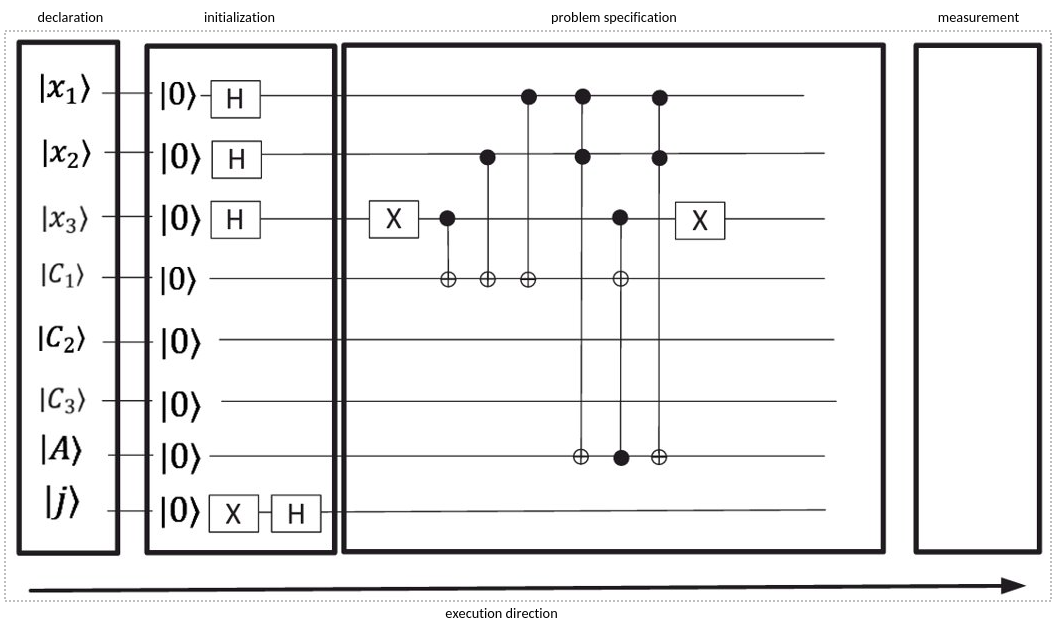
Creating a quantum circuit is a fundamental process in quantum computing. Following the figure above, this process can be broken down into several steps as follows:
Qubits Declaration: This is the first step in setting up a quantum program and it involves specifying the number of qubits to be used. By declaring qubits, we are essentially setting up 'variables' that will be used in the quantum program. Classical bits can also be declared, and they often come into play when we need to store and manipulate the results of quantum measurements. In addition, auxiliary qubits (also known as ancillary qubits) are often declared to assist in quantum computations. These are used as "scratch space" during computation or for holding temporary values, and they do not typically contain meaningful data at the end of the computation. Just like regular qubits, they are declared at the start of your quantum program.
Qubits Initialization: After declaring qubits, the next step is to initialize them. All qubits in a quantum computer start from the |0⟩ state, however, we can use quantum gates, such as the Hadamard gate, to initialize our qubits into a superposition state.
Problem Specification with Quantum Gates: After initializing the qubits, we then specify our problem in the form of a quantum circuit. A quantum circuit is a series of quantum gates (operations) that are applied to our qubits in a particular order to perform computations. The gates transform the initial state of the qubits into another state. Different problems will require different quantum circuits, and the design of these circuits is a crucial aspect of quantum algorithm design.
Measurement to Obtain Results: The final step in a quantum program involves measuring the qubits to obtain results. Measurements in quantum computing are unique because they not only give you the state of the qubits (either |0⟩ or |1⟩ for each qubit) but also collapse the quantum state to the measured state. The results of the measurement are then read out to classical bits, which can be further processed on a classical computer if necessary. This step allows us to extract useful information from the quantum system into the classical world.
Quantum program compilation and execution
Create Your Quantum Algorithm: The first step in quantum programming is very similar to classic programming - you have to come up with an algorithm. Instead of typical if... then... else... type instructions, you'll be working with a quantum circuit filled with quantum gates, which act as the basic instructions for your algorithm.
Choose Your Environment and Language: Next, you'll need to select an environment and programming language for writing your quantum code. Many beginners start with Python because of its simplicity and the availability of quantum libraries, such as Qiskit from IBM or QLM from ATOS.
Transpile Your Code: After writing your code, you'll need to convert (or transpile) it into a language that quantum computers understand - this is often QASM (Quantum Assembly Language). The transpiler not only translates your code but also optimizes it, ensuring your quantum circuit runs as efficiently as possible. This optimization takes into account the specific properties of the quantum machine that will run the code.
Execute Your Quantum Circuit: The final step is to run your quantum circuit. You can do this in two ways - either on a classic computer using a quantum simulator or on a real quantum machine. Running a circuit on a simulator is useful for testing and learning, as it allows you to experiment with "perfect" qubits without the hardware limitations or noise issues of real quantum computers. However, to fully experience the power of quantum computing, you may want to run your code on a real quantum machine. This is typically done by sending your code over the internet to a quantum computer service, like the one provided by IBM through Qiskit. Once received, your code is placed in a queue and executed when the machine is available.
Our scope for this tutorial
The main objective of the Quantum Computing simulation with R is to learn how to write quantum programs using the qsmulatR package. Thus we will only focus on point "2. Choose Your Environment and Language" above by converting our R code into Qiskit with the qsimulatR::export2qiskit() function.
Here's a quick & dirty implementation with qsimulatR for a very famous quantum algorithm, try to identify the initialization, the problem specification and the measurement parts. The algorithm will be explained in the next article.
x <- qstate(3)
x <- H(2)*(H(1)*x)
x <- H(3)*(X(3)*x)
x <- X(1) * (CCNOT(c(1,2,3)) *(X(1) * x))
for(i in c(1:3)) {
  x <- H(i) * x
}
x <- X(1) * (X(2) * x)
x <- cqgate(bits = c(1,2), gate = Z(2L)) * x
x <- X(1) * (X(2) * x)
for(i in c(1:2)) {
  x <- H(i) * x
}
x
qsimulatR::plot(x, qubitnames = c("x1", "x2", "j"))
hist(measure(e1 = x, bit = 2, repetitions = 1))
Remember, quantum programming can seem daunting at first, but with practice and patience, you'll start to grasp these new concepts and begin to appreciate the immense potential that quantum computing offers. Happy coding!
References
[1] Bourreau E., Fleury, G., Lacomme P., "Introduction à l'informatique quantique, Apprendre à calculer sur des ordinateurs quantiques avec Python", Collection Blanche, Eyrolles, 2022