
Grover's algorithm with qsimulatR
The groundwork for learning more complex quantum algorithms

Cover photo by gorodenkoff on iStock
Go to R-bloggers for R news and tutorials contributed by hundreds of R bloggers.
This is the fourth article of the Quantum Computing simulation with R series.
Introduction
Grover's algorithm, named after its inventor Lov Grover, is one of the foundational algorithms in quantum computing, and understanding it is crucial for several reasons:
Quantum Speedup: Grover's algorithm provides a practical demonstration of "quantum speedup." It's used for unstructured search problems and offers a significant speed advantage over classical algorithms. In a database with N items, Grover's algorithm can find a target item in roughly √N steps, compared to N/2 steps on average for a classical algorithm. This quadratic speedup exemplifies the computational potential* of quantum computing.
Amplitude Amplification: Grover's algorithm introduces the key concept of amplitude amplification, a technique used to increase the probability amplitude of the desired states. This is central not only to Grover's algorithm but also to other quantum algorithms.
Quantum Gates and Operations: Implementing Grover's algorithm helps understand the application of various quantum gates and their combined operations. It makes use of the Hadamard gate to create superposition, and phase inversion and amplitude amplification to manipulate these superpositions.
Quantum Advantage in Practice: While some quantum algorithms require a fully fault-tolerant quantum computer to demonstrate quantum advantage, Grover's algorithm can provide quantum speedup on near-term quantum devices, which makes it particularly important for practical quantum computing.
Basis for Other Algorithms: Understanding Grover's algorithm lays the groundwork for learning more complex quantum algorithms. Many advanced algorithms use principles demonstrated in Grover's algorithm, such as the amplitude amplification technique.
(*) Although Grover's algorithm requires the entire search space to be in superposition, which may not be feasible for certain large-scale practical applications, it remains an important example of quantum speedup, and understanding it is crucial to understanding many other quantum algorithms.
The Basics of Grover's Algorithm
Grover's algorithm is designed to address the problem of unstructured search. By "unstructured" search, we mean that the algorithm is designed to search through an unordered, unsorted, or random list of elements where no particular structure or relationship among the elements can be exploited to simplify the search.
Grover's algorithm is highly versatile and not restricted to problems with unique solutions. It can efficiently handle problems with multiple solutions, enhancing the probabilities associated with all solution states, thereby increasing the likelihood of measuring a correct answer upon executing the algorithm.
Grover's algorithm involves two main steps that are repeated iteratively: the application of the oracle function, and the application of the Grover diffusion operator (amplitude amplification). See the figure below from Figgat et al. [1].
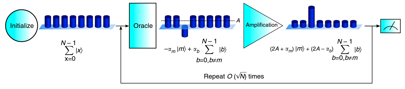
Here is a high-level overview of Grover's algorithm and its stages:
Initialization: The algorithm begins by initializing a quantum system of n qubits into a superposition of all possible states. This is done by applying a Hadamard gate to each qubit in the initial state |0>. As a result, we obtain an equal superposition of all 2^n possible states.
Oracle Application: In the second step, an "oracle" function is applied to the system. The oracle is a black box function that recognizes the solution(s) we are searching for. When it encounters a solution, it flips the sign of the state, leaving other states untouched. This marks the correct solution(s) with a phase difference.
Amplitude Amplification: After the oracle application, the amplitudes of the states are manipulated through a process called "amplitude amplification" or Grover diffusion operator. This process involves flipping the amplitudes of the states about the average amplitude, thus amplifying the amplitude (probability) of the marked state(s) while diminishing others.
Iteration: Steps 2 and 3 are iteratively repeated approximately √N times to increase the probability of measuring the marked state(s) (N is the total number of items in the list or the size of the search space).
Measurement: Finally, a measurement is performed. At this point, the system will most likely collapse into the marked state(s) — the solution(s) to the search problem.
Understanding the Oracle
An oracle, in the context of quantum computing, is a "black box" operation used in quantum algorithms that provides a solution to a specific problem instance. It's a key component in many quantum algorithms such as Grover's and Shor's algorithms. It encodes the problem we're trying to solve into a quantum state, and it can recognize a solution to the problem without revealing what the solution is.
In Grover's algorithm, the oracle is a function that marks the elements we are searching for. It's capable of recognizing whether a given input is a solution and flips the sign of the state if it is a solution.
The quantum oracle is implemented as a unitary transformation, which when applied to a particular quantum state, alters the state in some way dependent on the problem at hand. The rest of the quantum algorithm then uses this "marked" state to amplify the probability of measuring the system in the state corresponding to the solution, using the principles of quantum superposition and interference.
Oracles are hypothetical constructs used in the analysis of quantum algorithms. In practice, constructing an efficient oracle is often as hard as solving the problem itself classically. However, for certain problems, we can construct efficient quantum oracles, and this gives us quantum speedup over classical algorithms.
Example: 1-solution Grover algorithm
As an example, let's assume we have a list of four items, {0, 1, 2, 3}, and we know that item 2 is the solution to our problem. In binary representation, these items are {00, 01, 10, 11}. In this scenario, the quantum oracle will flip the sign of the amplitude of the state |10⟩ (which corresponds to item 2) while leaving all other states unchanged.
In quantum circuit terms, this can be realized by a controlled-Z gate acting on the two qubits of the system, with the target being the second qubit.
This process does not disclose the solution (item 2) to us directly, but it prepares the ground for the next stage of the algorithm, the amplitude amplification stage, which will make this solution more likely to be observed upon measurement.
When implementing Grover's algorithm for a problem with a unique solution, an extra qubit, often referred to as an "ancillary" or "auxiliary" qubit, is utilized. Therefore, we implement it on an (n+1)-qubit system, where the additional qubit assists in marking the solution state during the oracle operation.
# Here's the function that implements an oracle
# marking item 2 = |10> as the solution
oracle_item2 <- function(x){
# CCNOT = "controlled controlled NOT gate"
    x <- X(1) * (CCNOT(c(1,2,3))*(X(1) * x))
    return(x)
}

# item 1 = |00> + ancillary qubit => |000>
> item0 <- qstate(nbits = 2+1, coefs = c(1,0,0,0,0,0,0,0))
> item0
   ( 1 )    * |000>
# item 1 = |01> + ancillary qubit => |001>
> item1 <- qstate(nbits = 2+1, coefs = c(0,1,0,0,0,0,0,0))
> item1
   ( 1 )    * |001>
# item 2 = |10> + ancillary qubit => |010>
> item2 <- qstate(nbits = 2+1, coefs = c(0,0,1,0,0,0,0,0))
> item2 # the solution
   ( 1 )    * |010>
# item 3 = |11> + ancillary qubit => |011>
> item3 <- qstate(nbits = 2+1, coefs = c(0,0,0,1,0,0,0,0))
> item3
   ( 1 )    * |011>

# The oracle function flip the 3rd qubit (or bit 3) to |1>
> oracle_item2(item0)
   ( 1 )    * |000>
> oracle_item2(item1)
   ( 1 )    * |001>
> oracle_item2(item2) # the oracle marks item 2, bit 3 flipped to |1>
   ( 1 )    * |110>
> oracle_item2(item3)
   ( 1 )    * |011>

> measure(oracle_item2(item0), bit = 3)$value
[1] 0
> measure(oracle_item2(item1), bit = 3)$value
[1] 0
> measure(oracle_item2(item2), bit = 3)$value # solution
[1] 1
> measure(oracle_item2(item3), bit = 3)$value
[1] 0
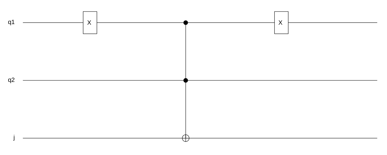
Now that we have verified that our oracle function oracle_item2 works, let us plot its circuit with any (2+1)-qubit system (nbits=3), here I used |000> as input. I also labeled the ancillary qubit as "j".
> qsimulatR::plot(oracle_item2(qstate(3)), qubitnames=c("q1","q2","j"))
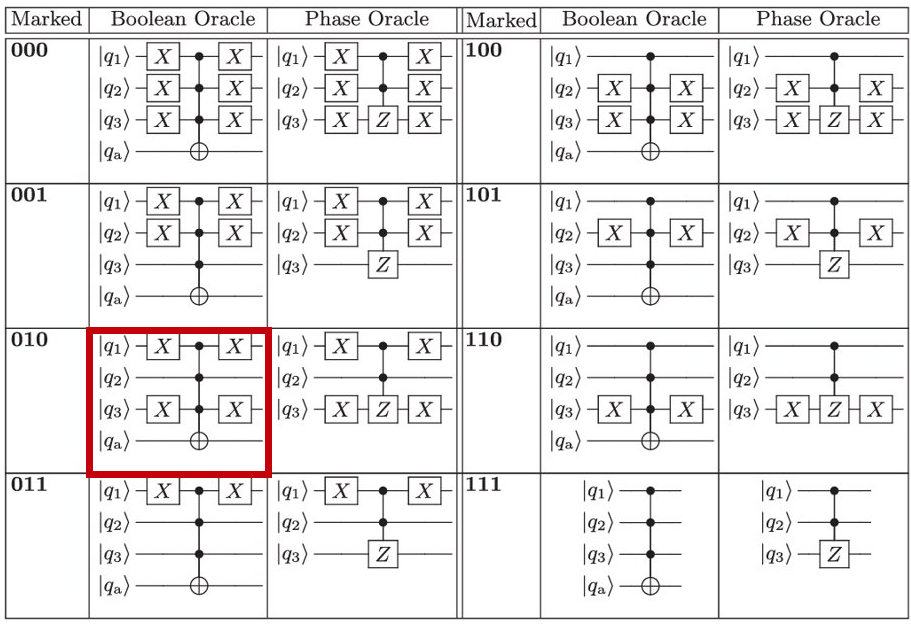
See the figure below from Figgat et al. article [1]. It shows 1-solution oracles for a (3+1)-qubit system. The red square shows the equivalent item2-oracle for 3 qubits e.g. marked solution = |010>.
Oracle - Mathematical explanation
For our previous (2+1)-qubit system with solution = item 2 = |10>, we usually write the oracle's output quantum state as
$$|\psi'> = \frac{1}{2}|00> +\frac{1}{2}|01> \textbf{-}\frac{1}{2}\textbf{|10>} +\frac{1}{2}|11>$$
Thus, the oracle marks the solution by flipping its sign. This corresponds to a phase flip that can be achieved with a Z gate on a single qubit, and this is why you see a "Phase Oracle" implementation in the figure above e.g. a Controlled-Z (CZ) gate can be used to implement an oracle in Grover's algorithm without the need for an ancillary qubit, assuming your problem is defined in such a way that a single CZ operation can correctly mark your solution state(s).
Note: here we stick to the "Boolean Oracle" implementation because we will also be working with more than two qubits or dealing with situations where the solution state isn't simply marked by a single CZ operation. Thus, a more complex oracle involving multiple gates (like CCNOTs, ancillary qubits, and additional phase gates) may be required.
That said, let's get back to this phase flip performed by the oracle from a mathematical perspective: the oracle function is essentially performing a symmetry operation e.g. implementing a reflection about the axis corresponding to the state |0>.
$$|\psi'> =\textbf{S}_{|0>}.|\psi>$$
$$|\psi'> =({2|0\gt\lt0| - I})(|\psi>)$$
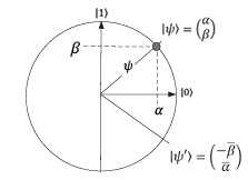
This symmetry is critical for the "amplitude amplification" process that follows the oracle operation in Grover's algorithm, where another reflection is performed about the superposition state, effectively amplifying the amplitudes of the solution state(s).
Grover diffusion operator
The Grover diffusion operator performs amplitude amplification is a procedure that manipulates these amplitudes to increase ("amplify") the amplitudes of desired states (i.e., solution states) while decreasing the amplitudes of undesired states. In essence, amplitude amplification increases the probability that a measurement will result in a desired state, making the correct solution more likely to be found when a measurement is made.
Thus, when the oracle is coupled with Grover's diffusion operator, the process iteratively moves the quantum system closer and closer to the desired solution state(s), improving the probability of measuring a solution when the quantum state is finally read out.
In the context of Grover's algorithm, amplitude amplification plays a crucial role in improving the algorithm's efficiency.
The combination of the oracle and the Grover diffusion operator forms the Grover iterator, and after approximately sqrt(N) iterations (where N is the total number of possible states), the quantum system is likely to be found in a solution state when a measurement is performed. Thus, Grover's algorithm can find a solution with high probability in O(sqrt(N)) steps, which is a significant speedup over classical algorithms that require O(N) steps for similar problems.
Here's a quick & dirty implementation of Grover's algorithm for item 2 = |10> as a solution, using qsimulatR.
# Initialization
x <- qstate(3)     # all 2+1 qubits initialized: |000>
x <- H(2)*(H(1)*x) # uniform superposition for bits 1 and 2
x <- H(3)*(X(3)*x) # ancillary qubit (bit 3) flipped to |1> before H
# Oracle function
x <- oracle_item2(x)
# Grover diffusiion
for(i in c(1:3)) {
  x <- H(i) * x
}
x <- X(1) * (X(2) * x)
x <- cqgate(bits = c(1,2), gate = Z(2L)) * x # custom CZ gate
x <- X(1) * (X(2) * x)
for(i in c(1:2)) {
  x <- H(i) * x
}
> x
   ( -1 )    * |110>
# N=2^2=4 is the special case where Grover's algorithm returns
# the correct result with certainty after only a single iteration
# Measure bit 1
> summary(measure(e1 = x, bit = 1)) # repetitions = 1 by default
Bit 1 has been measured 1 times with the outcome:
0:  1
1:  0
# Measure bit 2
> summary(measure(e1 = x, bit = 2))
Bit 2 has been measured 1 times with the outcome:
0:  0
1:  1
> allStatesProbabilities(x) # custom function, see previous article
|000> |001> |010> |011> |100> |101> |110> |111>
    0     0     0     0     0     0     1     0  # Prob('10')=1
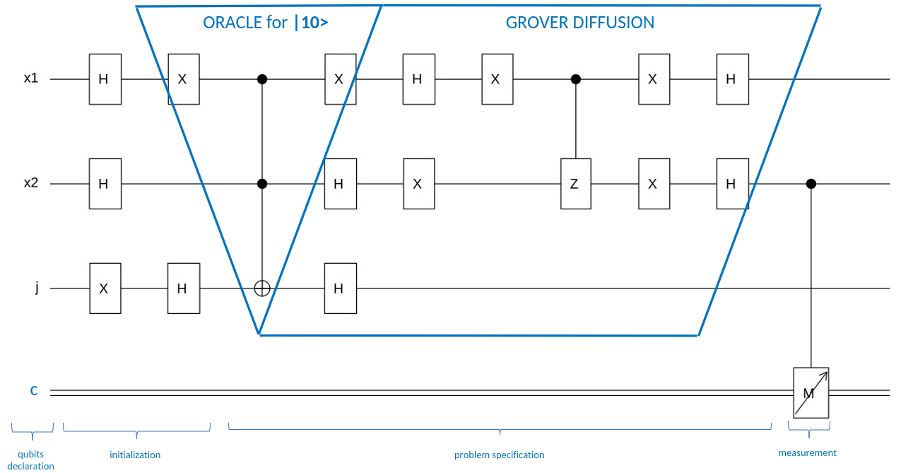
Let us plot Grover's algorithm final circuit for our example. I've added some comments manually (in blue) in the figure.
# The second qubit is measured and its value is stored in res$value
> res <- measure(e1 = x, bit = 2)
> res$value
[1] 1
# The wave function of the quantum state collapses,
# the result of which is stored again as a qstate object in res$psi.
> qsimulatR::plot(res$psi, qubitnames = c("x1", "x2", "j"))
Grover diffusion operator - Mathematical explanation
The Grover diffusion operator effectively performs a reflection of the state vector about the mean amplitude. Imagine that each state in your superposition is a point in your high-dimensional state space, and the average amplitude of all states forms another point in that space. The diffusion operator "reflects" each point about this average point. In the two-dimensional case, this would be like reflecting a point about a line in a plane.
$$|\phi> =\textbf{S}|\psi>.|\psi'> =\textbf{S}|\psi>.(S_{|0>}.|\psi>)$$
$$|\phi> =(2|{\psi\gt\lt\psi|} - I)(S_{|0>}.{|\psi>})$$
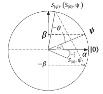
In summary [2], for the first iteration:
Superposition of |ψ⟩ => angle θ/2 between |ψ⟩ and |0⟩
Oracle function (symmetry) => angle -θ/2 with respect to |0⟩
Grover's diffusion operator (symmetry) => angle 3θ/2 with respect to |0⟩
Next iteration:
Oracle function (symmetry) => angle -3θ/2 with respect to |0⟩
Grover's diffusion operator (symmetry) => angle 5θ/2 with respect to |0⟩
Convert to Qiskit
Let us convert to Qiskit the result of the quantum state collapse res$psi with the qsimulatR export2qiskit function.
A circuit.py file will be created in the working directory. Important: the Qiskit Python code will not work! you need to perform some manual updates:
> res$psi
   ( -1 )    * |110>
# check @ circuit in str(x)
> export2qiskit(res$psi)
# automatically generated by qsimulatR
qc = QuantumCircuit(3,1) # we want 2 classical bits for measurement
qc.h(0)
qc.h(1)
qc.x(2)
qc.h(2)
qc.x(0)
qc.ccx(0, 1, 2)
qc.x(0)
qc.h(0)
qc.h(1)
qc.h(2)
qc.x(1)
qc.x(0)
qc.z(0, 1) # error: because custom cqgate() export is not supported
qc.x(1)
qc.x(0)
qc.h(0)
qc.h(1)
qc.measure(1, 0) # we want to measure index 0 and index 1 resp.
Below I've provided the updated Qiskit code with corrections as comments (# new)
# new: imports
from qiskit import *
from qiskit.visualization import plot_histogram
# automatically generated by qsimulatR
qc = QuantumCircuit(3,2) # new
qc.h(0)
qc.h(1)
qc.x(2)
qc.h(2)
qc.x(0)
qc.ccx(0, 1, 2)
qc.x(0)
qc.h(0)
qc.h(1)
qc.h(2)
qc.x(1)
qc.x(0)
qc.ccz(0, 1, 2) # new: replaced by ccz gate
qc.x(1)
qc.x(0)
qc.h(0)
qc.h(1)
# new: Measure the first two qubits into the classical bits
qc.measure(0,0)
qc.measure(1,1)
# new: draw the circuit
qc.draw()

# ... Cont'd
# new: job execution with simulator backend
backend = BasicAer.get_backend('qasm_simulator')
job = execute(qc, backend)
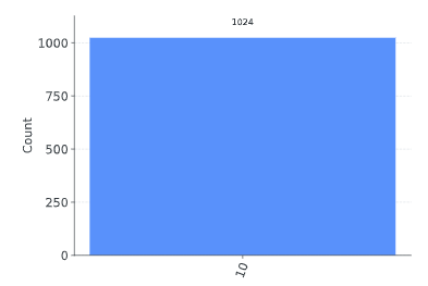
job.result().get_counts() # result: {'10': 1024}
plot_histogram(job.result().get_counts())
Before concluding
As we delve into the fascinating world of quantum computing and begin to grapple with concepts such as Grover's algorithm, it's perfectly natural for certain questions to arise.
You might wonder, for example, why we initialize the ancillary 'j' qubit to |1>?, or why we use a CCZ gate and additional gates for the Grover diffusion process?
Remember, at this stage of our exploration, we are focusing on the key principles and operations without getting too lost in the mathematical underpinnings. These aspects are influenced by specific quantum mechanical properties and mathematical considerations that ensure the algorithm's optimal performance.
However, rest assured that as we progress in our quantum computing journey, and as your understanding deepens, these concepts will become more intuitive. The goal right now is to build a solid foundation, encourage curiosity, and nurture a passion for this transformative field.
Conclusion
In conclusion, Grover's algorithm, a cornerstone in quantum computing, provides an extraordinary advantage for unstructured search, making it an essential topic for those venturing into this field. The beauty of this algorithm lies in its simplicity and the fundamental quantum principles it employs, such as superposition, interference, and quantum entanglement.
In this article, we've explored the key elements that make Grover's algorithm tick, including the creation of a specific quantum oracle and the Grover diffusion operator, which is responsible for the algorithm's amplitude amplification process. By doing so, we've dived into the depth of the algorithm, visualizing it not just as a sequence of gates but rather as a dance of symmetries in the quantum space.
Alongside the theoretical understanding, we've delved into practical implementation using the qsimulatR package in R and how to convert our code to Qiskit. This exercise enhances our comprehension of the algorithm and gives us the hands-on experience necessary to embark on more complex quantum computing problems.
As we continue our journey in quantum computing, keep in mind that the principles and techniques employed in Grover's algorithm echo through many other quantum algorithms. Therefore, a solid grasp of this topic forms a vital stepping stone in your quantum computing journey.
References
[1] Figgat C., Maslov D., Landsman K.A., Linke N.M., Debnath S., Monroe C., "Complete 3-Qubit Grover search on a programmable quantum computer", Nature Communications, 8:1918|DOI:10.1038/s41467-017-01904-7| www.nature.com/naturecommunications, 2017
[2] Bourreau E., Fleury, G., Lacomme P., "Introduction à l'informatique quantique, Apprendre à calculer sur des ordinateurs quantiques avec Python", Collection Blanche, Eyrolles, 2022