# Time Series Forecasting Lab (Part 5) - Ensembles
Cover photo by Hannah Busing on Unsplash
Go to [R-bloggers](https://www.r-bloggers.com/) for R news and tutorials contributed by hundreds of R bloggers.
## Introduction
This is the fifth of a series of 6 articles about time series forecasting with panel data and ensemble stacking with R.
Through these articles I will be putting into practice what I have learned from the Business Science University training course [1](https://university.business-science.io/courses) DS4B 203-R: High-Performance Time Series Forecasting", delivered by Matt Dancho. If you are looking to gain a high level of expertise in time series with R I strongly recommend this course.
The objective of this article is learn how to create average and weighted ensembles using all (both non-tuned and tuned) model from [Part 3](https://blog.bguarisma.com/time-series-forecasting-and-ensemble-stacking-part-3) and [Part 4](https://blog.bguarisma.com/time-series-forecasting-and-ensemble-stacking-part-4). We will also check if any of these ensemble models can outperform the tuned Prophet Boost model.
### Prerequisites
I assume you are already familiar with the following topics, packages and terms:
- dplyr or tidyverse R packages
- calibration table from [Part 3](https://blog.bguarisma.com/time-series-forecasting-and-ensemble-stacking-part-3) and [Part 4](https://blog.bguarisma.com/time-series-forecasting-and-ensemble-stacking-part-4)
- model evaluation metrics: RMSE, R-squared, ...
## Packages
The following packages must be loaded:
```
# 01 FEATURE ENGINEERING
library(tidyverse) # loading dplyr, tibble, ggplot2, .. dependencies
library(timetk) # using timetk plotting, diagnostics and augment operations
library(tsibble) # for month to Date conversion
library(tsibbledata) # for aus_retail dataset
library(fastDummies) # for dummyfying categorical variables
library(skimr) # for quick statistics
# 02 FEATURE ENGINEERING WITH RECIPES
library(tidymodels) # with workflow dependency
# 03 MACHINE LEARNING
library(modeltime) # ML models specifications and engines
library(tictoc) # measure training elapsed time
# 04 HYPERPARAMETER TUNING
library(future)
library(doFuture)
library(plotly)
# 05 ENSEMBLES
library(modeltime.ensemble)
```
## Load calibration tables
Load all calibration tables for all tuned & non-tuned models we have trained so far, nad remind ourselves of the accuracy results so far:
```
> calibration_tbl <- read_rds("workflows_NonandTuned_artifacts_list.rds")
> calibration_tbl <- calibration_tbl$calibration
> calibration_tbl %>%
modeltime_accuracy() %>%
arrange(rmse)
# A tibble: 8 x 9
.model_id .model_desc .type mae mape mase smape rmse rsq
1 7 PROPHET W/ REGRESSORS Test 0.189 21.6 0.417 21.5 0.240 0.856
2 3 PROPHET W/ REGRESSORS - Tuned Test 0.189 21.6 0.418 21.5 0.241 0.857
3 4 PROPHET W/ XGBOOST ERRORS - Tuned Test 0.191 25.7 0.421 19.9 0.253 0.780
4 8 PROPHET W/ XGBOOST ERRORS Test 0.204 24.8 0.451 20.8 0.287 0.753
5 2 XGBOOST - Tuned Test 0.219 23.6 0.482 22.9 0.296 0.762
6 6 XGBOOST Test 0.216 25.0 0.476 22.4 0.299 0.747
7 1 RANGER - Tuned Test 0.231 26.1 0.509 24.6 0.303 0.766
8 5 RANGER Test 0.235 25.4 0.519 25.0 0.312 0.765
```
## Average ensembles
Average ensembles is a fairly simple concept, its main advantage is that it does not require retraining. If you use the **mean** be aware of the individual performance of each model since the "average model" performance will be sensitive to "bad models" and outliers. To cope with this situation you can use the **median** (more robust than the mean). Do not use the median when all models are doing pretty well.
To create these two ensembles is pretty simple, all you have to do is to pipe the modeltime table with all workflows into the ```ensemble_average()``` and specify the ```type```, either mean or median.
```
> ensemble_fit_mean <- submodels_tbl %>%
ensemble_average(type = "mean")
> ensemble_fit_mean
-- Modeltime Ensemble -------------------------------------------
Ensemble of 8 Models (MEAN)
# Modeltime Table
# A tibble: 8 x 5
.model_id .model .model_desc .type .calibration_data
1 1 RANGER - Tuned Test
2 2 XGBOOST - Tuned Test
3 3 PROPHET W/ REGRESSORS - Tuned Test
4 4 PROPHET W/ XGBOOST ERRORS - Tuned Test
5 5 RANGER Test
6 6 XGBOOST Test
7 7 PROPHET W/ REGRESSORS Test
8 8 PROPHET W/ XGBOOST ERRORS Test
> ensemble_fit_mean <- submodels_tbl %>%
ensemble_average(type = "median")
-- Modeltime Ensemble -------------------------------------------
Ensemble of 8 Models (MEDIAN)
# Modeltime Table
# A tibble: 8 x 5
.model_id .model .model_desc .type .calibration_data
1 1 RANGER - Tuned Test
2 2 XGBOOST - Tuned Test
3 3 PROPHET W/ REGRESSORS - Tuned Test
4 4 PROPHET W/ XGBOOST ERRORS - Tuned Test
5 5 RANGER Test
6 6 XGBOOST Test
7 7 PROPHET W/ REGRESSORS Test
8 8 PROPHET W/ XGBOOST ERRORS Test
```
## Weigthed ensembles

Weighted ensembles can improve performance compared to average ensembles but we must decide of the weight values. One solution is to use a simple *rank technique*: create a rank column for which highest value is for the best model (lowest RMSE).
In the code snippet below we add the ```rank``` column and then we select ```.model_id``` and ```rank``` columns to define a loadings tibble which will be used for defining the weighted ensemble.
```
> calibration_tbl %>%
modeltime_accuracy() %>%
mutate(rank = min_rank(-rmse))
# A tibble: 8 x 10
.model_id .model_desc .type mae mape mase smape rmse rsq rank
1 1 RANGER - Tuned Test 0.231 26.1 0.509 24.6 0.303 0.766 2
2 2 XGBOOST - Tuned Test 0.219 23.6 0.482 22.9 0.296 0.762 4
3 3 PROPHET W/ REGRESSORS - Tuned Test 0.189 21.6 0.418 21.5 0.241 0.857 7
4 4 PROPHET W/ XGBOOST ERRORS - Tuned Test 0.191 25.7 0.421 19.9 0.253 0.780 6
5 5 RANGER Test 0.235 25.4 0.519 25.0 0.312 0.765 1
6 6 XGBOOST Test 0.216 25.0 0.476 22.4 0.299 0.747 3
7 7 PROPHET W/ REGRESSORS Test 0.189 21.6 0.417 21.5 0.240 0.856 8
8 8 PROPHET W/ XGBOOST ERRORS Test 0.204 24.8 0.451 20.8 0.287 0.753 5
> loadings_tbl <- submodels_tbl %>%
modeltime_accuracy() %>%
mutate(rank = min_rank(-rmse)) %>%
select(.model_id, rank)
```
Then the weigths are created by passing models' rank to the ```ensemble_weighted()``` function. The newly created ".loadings" column are the weights, the sum of all weigths is equal to 1.
```
> ensemble_fit_wt <- submodels_tbl %>%
ensemble_weighted(loadings = loadings_tbl$rank)
> ensemble_fit_wt$fit$loadings_tbl
# Modeltime Table
# A tibble: 8 x 2
.model_id .loadings
1 1 0.0556
2 2 0.111
3 3 0.194
4 4 0.167
5 5 0.0278
6 6 0.0833
7 7 0.222
8 8 0.139
```
## Models evaluation
Finally, let us display the accuracy results by adding previous ensemble models to a modeltime table, calibrating the latter and piping it into the ```modeltime_accuracy()``` function. We sort by ascending RMSE.
```
modeltime_table(
ensemble_fit_mean,
ensemble_fit_median,
ensemble_fit_wt
) %>%
modeltime_calibrate(testing(splits)) %>%
modeltime_accuracy(testing(splits)) %>%
arrange(rmse)
# A tibble: 3 x 9
.model_id .model_desc .type mae mape mase smape rmse rsq
1 3 ENSEMBLE (WEIGHTED): 8 MODELS Test 0.176 20.7 0.388 19.5 0.237 0.840
2 1 ENSEMBLE (MEAN): 8 MODELS Test 0.189 21.8 0.417 20.6 0.255 0.819
3 2 ENSEMBLE (MEDIAN): 8 MODELS Test 0.204 23.0 0.450 21.8 0.275 0.797
```
As per the table below the **weighted average ensemble** performs better than other two average ensembles.
Let us now check if it performs better than the individual workflows from [Part 4](https://blog.bguarisma.com/time-series-forecasting-and-ensemble-stacking-part-4).
We add the ensembles' calibration table to the non-tuned and tuned models' calibration table (```calibration_tbl```).
```
> calibration_all_tbl <- modeltime_table(
ensemble_fit_mean,
ensemble_fit_median,
ensemble_fit_wt
) %>%
modeltime_calibrate(testing(splits)) %>%
combine_modeltime_tables(calibration_tbl)
> calibration_all_tbl %>%
modeltime_accuracy() %>%
arrange(rmse)
# A tibble: 11 x 9
.model_id .model_desc .type mae mape mase smape rmse rsq
1 3 ENSEMBLE (WEIGHTED): 8 MODELS Test 0.176 20.7 0.388 19.5 0.237 0.840
2 10 PROPHET W/ REGRESSORS Test 0.189 21.6 0.417 21.5 0.240 0.856
3 6 PROPHET W/ REGRESSORS - Tuned Test 0.189 21.6 0.418 21.5 0.241 0.857
4 7 PROPHET W/ XGBOOST ERRORS - Tuned Test 0.191 25.7 0.421 19.9 0.253 0.780
5 1 ENSEMBLE (MEAN): 8 MODELS Test 0.189 21.8 0.417 20.6 0.255 0.819
6 2 ENSEMBLE (MEDIAN): 8 MODELS Test 0.204 23.0 0.450 21.8 0.275 0.797
7 11 PROPHET W/ XGBOOST ERRORS Test 0.204 24.8 0.451 20.8 0.287 0.753
8 5 XGBOOST - Tuned Test 0.219 23.6 0.482 22.9 0.296 0.762
9 9 XGBOOST Test 0.216 25.0 0.476 22.4 0.299 0.747
10 4 RANGER - Tuned Test 0.231 26.1 0.509 24.6 0.303 0.766
11 8 RANGER Test 0.235 25.4 0.519 25.0 0.312 0.765
```
## Forescast plot
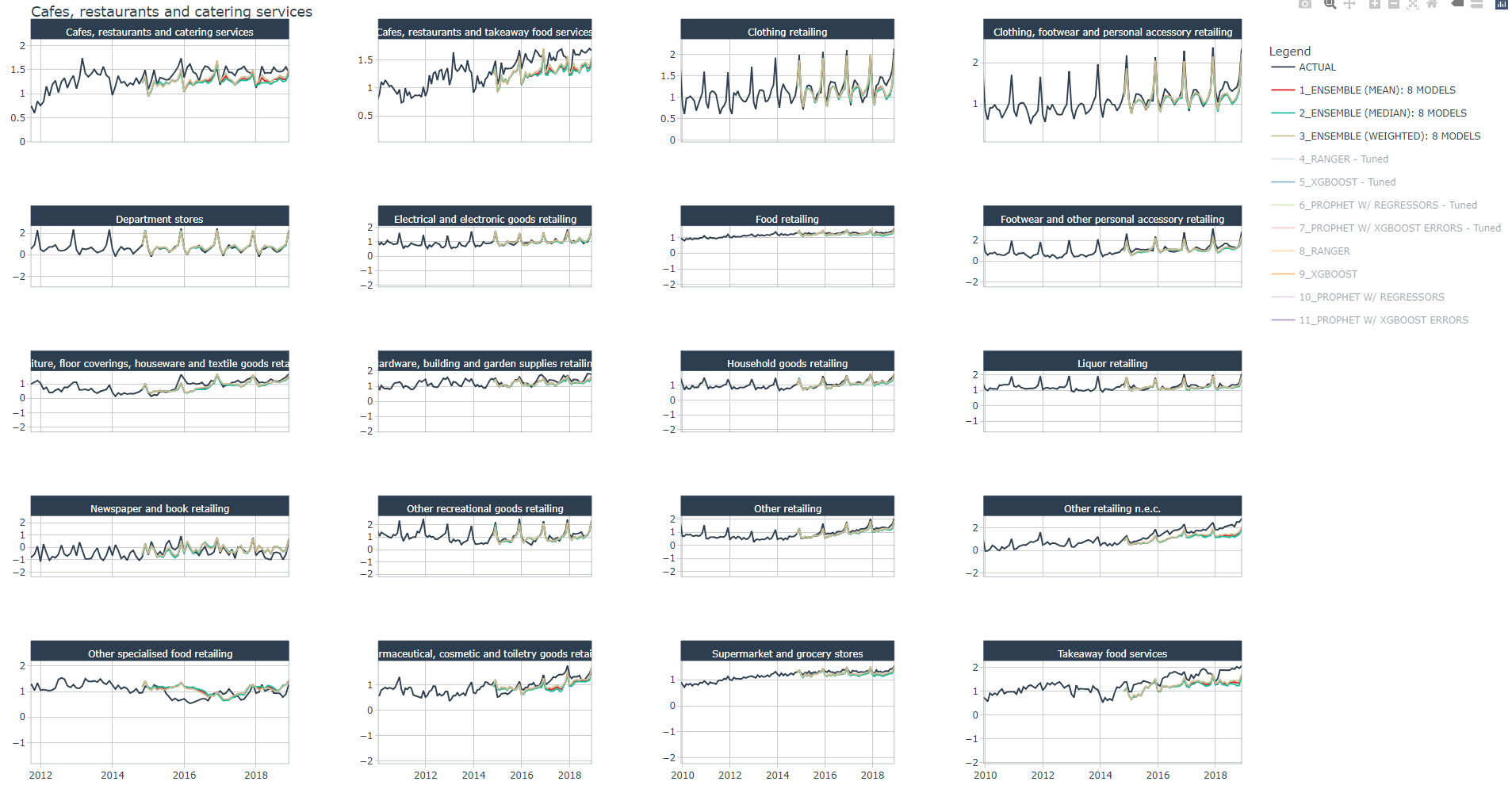
We have already plotted all tuned and non-tuned models' forecast in [Part 4](https://blog.bguarisma.com/time-series-forecasting-lab-part-4-hyperparameter-tuning), here we plot only the average ensembles' forecast.
## Conclusion
In this article you've learned how to create **average (mean or median) ensembles** and **weighted average ensembles**. The latter was created using the rank technique.
Since one of the average ensemble was the best model, we did not bother with improving ensemble models' performance with **model selection** e.g., selecting the **top 5 models** and/or **suppressing redundant models** such as the tuned and non-tuned Prophet models which have the same performance.
In Part 5, we will try to outperform the weighted average ensemble .
## References
[1](https://university.business-science.io/courses) Dancho, Matt, "*DS4B 203-R: High-Performance Time Series Forecasting*", Business Science University