# Time Series Forecasting Lab (Part 3) - Machine Learning with Workflows
Cover photo by Solen Feyissa on Unsplash
Go to [R-bloggers](https://www.r-bloggers.com/) for R news and tutorials contributed by hundreds of R bloggers.
## Introduction
This is the third of a [series](https://blog.bguarisma.com/series/time-series-forecasting) of 6 articles about time series forecasting with panel data and ensemble stacking with R.
Through these articles I will be putting into practice what I have learned from the Business Science University training course [2](https://university.business-science.io/courses) DS4B 203-R: High-Performance Time Series Forecasting", delivered by Matt Dancho. If you are looking to gain a high level of expertise in time series with R I strongly recommend this course.
The objective of this article is to show how do we fit machine learning models for time series with [modeltime](https://business-science.github.io/modeltime/). Modeltime is used to integrate time series models ino the tydimodels ecosystem.
You will understand the notion of forecasting [workflows](https://workflows.tidymodels.org/) e.g., how to fit a model by adding its **specification **and corresponding preprocessing **recipe** (see [Part 2](https://blog.bguarisma.com/time-series-forecasting-and-ensemble-stacking-part-2) ) to a workflow. The notion of **modeltime table** and **calibration table** will also be very useful since it allows to evaluate and forecast all models at the same time for all time series (panel data). Finally, you will perform and plot forecasts on test dataset. Hyperparameter tuning will be covered in the next article ([Part 4](https://blog.bguarisma.com/time-series-forecasting-lab-part-4-hyperparameter-tuning)).
### Prerequisites
I assume you are already familiar with the following topics, packages and terms:
- dplyr or tidyverse R packages
- Random Forest, XGBoost, Prophet, Prophet Boost algorithms
- notion of recipes for time series (timetk, see [Part 2](https://blog.bguarisma.com/time-series-forecasting-and-ensemble-stacking-part-2))
- model evaluation metrics: RMSE, R-squared, ...
## Packages
The following packages must be loaded:
```
# 01 FEATURE ENGINEERING
library(tidyverse) # loading dplyr, tibble, ggplot2, .. dependencies
library(timetk) # using timetk plotting, diagnostics and augment operations
library(tsibble) # for month to Date conversion
library(tsibbledata) # for aus_retail dataset
library(fastDummies) # for dummyfying categorical variables
library(skimr) # for quick statistics
# 02 FEATURE ENGINEERING WITH RECIPES
library(tidymodels) # with workflow dependency
# 03 MACHINE LEARNING
library(modeltime) # ML models specifications and engines
library(tictoc) # measure training elapsed time
```
## Fitting ML models
As depicted in the figure below, the end-to-end process is the following:
1. define 4 workflows, each comprising the model specification and engine, the recipe (can be updated), and the fit function on the training dataset extracted from the splits object.
2. add all workflows into a modeltime table and calibrate
3. evaluate models based on default performance metrics
4. perform and plot forecasts with test dataset

### Load artifacts
Let us load our work from Part 2.
```
artifacts <- read_rds("feature_engineering_artifacts_list.rds")
splits <- artifacts$splits
recipe_spec <- artifacts$recipes$recipe_spec
Industries <- artifacts$data$industries
```
#### Check training data
Remember, the training data is not ```trainings(data)```, it is the output of the recipe specification ```recipe_spec``` once you *prepare* it and *juice* it, as shown in the code snippet below :
```
> recipe_spec %>%
prep() %>%
juice() %>%
glimpse()
Rows: 6,840
Columns: 52
$ rowid 14, 467, 920, 1373, 1826, 2279, 2732, ~
$ Month 1983-05-01, 1983-05-01, 1983-05-01, 1~
$ Month_sin12_K1 0.5145554, 0.5145554, 0.5145554, 0.514~
$ Month_cos12_K1 8.574571e-01, 8.574571e-01, 8.574571e-~
$ Turnover_lag12 -2.355895, -2.397538, -1.674143, -1.89~
$ Turnover_lag13 -2.011144, -2.195619, -1.713772, -1.89~
$ Turnover_lag12_roll_3 -2.216035, -2.299396, -1.771137, -1.97~
$ Turnover_lag13_roll_3 -2.183520, -2.296579, -1.693957, -1.89~
$ Turnover_lag12_roll_6 -2.213974, -2.275130, -1.824439, -2.02~
$ Turnover_lag13_roll_6 -2.197201, -2.278793, -1.787835, -1.98~
$ Turnover_lag12_roll_9 -2.190758, -2.244673, -1.826687, -2.01~
$ Turnover_lag13_roll_9 -2.213974, -2.275130, -1.824439, -2.02~
$ Turnover_lag12_roll_12 -2.095067, -2.152525, -1.819038, -1.97~
$ Turnover_lag13_roll_12 -2.147914, -2.200931, -1.828293, -2.00~
$ Turnover -2.042611, -1.866127, -1.383977, -1.53~
$ Month_index.num -1.727262, -1.727262, -1.727262, -1.72~
$ Month_year -1.710287, -1.710287, -1.710287, -1.71~
$ Month_half 1, 1, 1, 1, 1, 1, 1, 1, 1, 1, 1, 1, 1,~
$ Month_quarter 2, 2, 2, 2, 2, 2, 2, 2, 2, 2, 2, 2, 2,~
$ Month_month 5, 5, 5, 5, 5, 5, 5, 5, 5, 5, 5, 5, 5,~
$ Industry_Cafes..restaurants.and.catering.services 1, 0, 0, 0, 0, 0, 0, 0, 0, 0, 0, 0, 0,~
$ Industry_Cafes..restaurants.and.takeaway.food.services 0, 1, 0, 0, 0, 0, 0, 0, 0, 0, 0, 0, 0,~
$ Industry_Clothing.retailing 0, 0, 1, 0, 0, 0, 0, 0, 0, 0, 0, 0, 0,~
$ Industry_Clothing..footwear.and.personal.accessory.retailing 0, 0, 0, 1, 0, 0, 0, 0, 0, 0, 0, 0, 0,~
$ Industry_Department.stores 0, 0, 0, 0, 1, 0, 0, 0, 0, 0, 0, 0, 0,~
$ Industry_Electrical.and.electronic.goods.retailing 0, 0, 0, 0, 0, 1, 0, 0, 0, 0, 0, 0, 0,~
$ Industry_Food.retailing 0, 0, 0, 0, 0, 0, 1, 0, 0, 0, 0, 0, 0,~
$ Industry_Footwear.and.other.personal.accessory.retailing 0, 0, 0, 0, 0, 0, 0, 1, 0, 0, 0, 0, 0,~
$ Industry_Furniture..floor.coverings..houseware.and.textile.goods.retailing 0, 0, 0, 0, 0, 0, 0, 0, 1, 0, 0, 0, 0,~
$ Industry_Hardware..building.and.garden.supplies.retailing 0, 0, 0, 0, 0, 0, 0, 0, 0, 1, 0, 0, 0,~
$ Industry_Household.goods.retailing 0, 0, 0, 0, 0, 0, 0, 0, 0, 0, 1, 0, 0,~
$ Industry_Liquor.retailing 0, 0, 0, 0, 0, 0, 0, 0, 0, 0, 0, 1, 0,~
$ Industry_Newspaper.and.book.retailing 0, 0, 0, 0, 0, 0, 0, 0, 0, 0, 0, 0, 1,~
$ Industry_Other.recreational.goods.retailing 0, 0, 0, 0, 0, 0, 0, 0, 0, 0, 0, 0, 0,~
$ Industry_Other.retailing 0, 0, 0, 0, 0, 0, 0, 0, 0, 0, 0, 0, 0,~
$ Industry_Other.retailing.n.e.c. 0, 0, 0, 0, 0, 0, 0, 0, 0, 0, 0, 0, 0,~
$ Industry_Other.specialised.food.retailing 0, 0, 0, 0, 0, 0, 0, 0, 0, 0, 0, 0, 0,~
$ Industry_Pharmaceutical..cosmetic.and.toiletry.goods.retailing 0, 0, 0, 0, 0, 0, 0, 0, 0, 0, 0, 0, 0,~
$ Industry_Supermarket.and.grocery.stores 0, 0, 0, 0, 0, 0, 0, 0, 0, 0, 0, 0, 0,~
$ Industry_Takeaway.food.services 0, 0, 0, 0, 0, 0, 0, 0, 0, 0, 0, 0, 0,~
$ Month_month.lbl_01 0, 0, 0, 0, 0, 0, 0, 0, 0, 0, 0, 0, 0,~
$ Month_month.lbl_02 0, 0, 0, 0, 0, 0, 0, 0, 0, 0, 0, 0, 0,~
$ Month_month.lbl_03 0, 0, 0, 0, 0, 0, 0, 0, 0, 0, 0, 0, 0,~
$ Month_month.lbl_04 0, 0, 0, 0, 0, 0, 0, 0, 0, 0, 0, 0, 0,~
$ Month_month.lbl_05 1, 1, 1, 1, 1, 1, 1, 1, 1, 1, 1, 1, 1,~
$ Month_month.lbl_06 0, 0, 0, 0, 0, 0, 0, 0, 0, 0, 0, 0, 0,~
$ Month_month.lbl_07 0, 0, 0, 0, 0, 0, 0, 0, 0, 0, 0, 0, 0,~
$ Month_month.lbl_08 0, 0, 0, 0, 0, 0, 0, 0, 0, 0, 0, 0, 0,~
$ Month_month.lbl_09 0, 0, 0, 0, 0, 0, 0, 0, 0, 0, 0, 0, 0,~
$ Month_month.lbl_10 0, 0, 0, 0, 0, 0, 0, 0, 0, 0, 0, 0, 0,~
$ Month_month.lbl_11 0, 0, 0, 0, 0, 0, 0, 0, 0, 0, 0, 0, 0,~
$ Month_month.lbl_12 0, 0, 0, 0, 0, 0, 0, 0, 0, 0, 0, 0, 0,~
```
### Notion of workflow
As per [workflows](https://workflows.tidymodels.org/), "A workflow is an object that can bundle together your pre-processing, modeling, and post-processing requests. The recipe prepping and model fitting can be executed using a single call to fit()".
The following code snippet is a template of a workflow definition:
```
wflw_fit_ <- workflow() %>%
add_model(
spec = (
) %>%
set_engine()
) %>%
add_recipe( ) %>%
fit(training(splits))
```
- initialize with ```workflow()``` the workflow that combines both a model and a preprocessing recipe.
- add the ML model specification to the workflow with ```add_model```
- set the correspondant engine with ```set_engine```
- add the recipe with ```add_recipe``` e.g., adds a preprocessing specification to the workflow
- if necessary, update recipe with recipes functions such as ```update_role()```, ```step_rm()```, etc. (see [Part 2](https://blog.bguarisma.com/time-series-forecasting-lab-part-2-feature-engineering-with-recipes))
- fit the model with ```fit(training(splits))```
### ML model specification and engine
You will find in the figure below the specification and engine(s) for each of the 4 models used in this article.
- Random Forest modeltime function ```rand_forest()``` uses ```ranger``` from [parsnip](https://parsnip.tidymodels.org/) package as default engine.
- XGBoost modeltime function ```boost_tree()``` uses ```xgboost``` from [parsnip](https://parsnip.tidymodels.org/) package as default engine.
- Prophet modeltime function ```prophet_reg()``` uses ```prophet``` from [modeltime](https://business-science.github.io/modeltime/) package as default engine.
- Prophet Boost modeltime function ```prophet_boost()``` uses ```prophet_xgboost ``` from [modeltime](https://business-science.github.io/modeltime/) package as default engine.
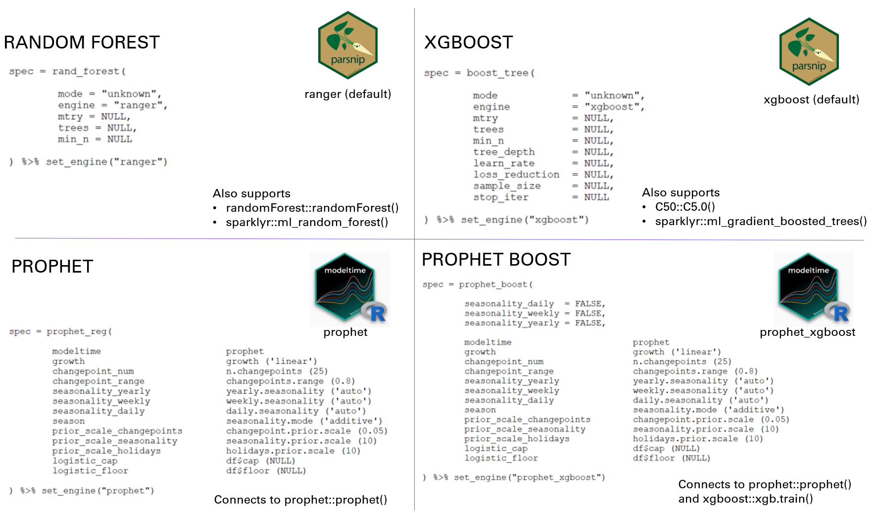
In this article **we will keep default specification values**, except for ```prophet()``` and ```prophet_xgboost()``` where we will make some modifications.
We will also measure the elapsed training time with ```titoc``` package. I'm using a Lenovo Windows 10 laptop, 16GB RAM, i5 CPU.
### Random Forest
You only need to indicate the ```mode``` in the specification. Since we are dealing with prdictions of a numeric measure (here ```Turnover```) the mode is a regression and not a classification.
For random forest, you need to update the recipe since ```rand_forest()``` will also consider ```Month``` (the timestamp) as a feature.
Code update: ```update_role()``` doesn't work with Data features, you must replace by ```step_rm()```
```
# * RANDOM FOREST ----
> tic()
wflw_fit_rf <- workflow() %>%
add_model(
spec = rand_forest(
mode = "regression"
) %>%
set_engine("ranger")
) %>%
add_recipe(recipe_spec %>%
step_rm(Month) %>%
fit(training(splits))
toc()
10.2 sec elapsed
> wflw_fit_rf
== Workflow [trained] =====================================================================================================
Preprocessor: Recipe
Model: rand_forest()
-- Preprocessor -----------------------------------------------------------------------------------------------------------
5 Recipe Steps
* step_other()
* step_timeseries_signature()
* step_rm()
* step_dummy()
* step_normalize()
-- Model ------------------------------------------------------------------------------------------------------------------
Ranger result
Call:
ranger::ranger(x = maybe_data_frame(x), y = y, num.threads = 1, verbose = FALSE, seed = sample.int(10^5, 1))
Type: Regression
Number of trees: 500
Sample size: 6840
Number of independent variables: 49
Mtry: 7
Target node size: 5
Variable importance mode: none
Splitrule: variance
OOB prediction error (MSE): 0.03631029
R squared (OOB): 0.952689
```
### XGBoost
You only need to indicate the ```mode``` in the specification. Since we are dealing with time series forecast of a numeric measure (here ```Turnover```) the mode is a regression and not a classification.
You need to update the recipe since ```boost_tree()``` will also consider ```Month``` (the timestamp) as a feature.
Code update: ```update_role()``` doesn't work with Data features, you must replace by ```step_rm()```
```
# * XGBOOST ----
tic()
wflw_fit_xgboost <- workflow() %>%
add_model(
spec = boost_tree(
mode = "regression"
) %>%
set_engine("xgboost")
) %>%
add_recipe(recipe_spec %>%
step_rm(Month) %>%
fit(training(splits))
toc()
1.06 sec elapsed
> wflw_fit_xgboost
== Workflow [trained] =====================================================================================================
Preprocessor: Recipe
Model: boost_tree()
-- Preprocessor -----------------------------------------------------------------------------------------------------------
5 Recipe Steps
* step_other()
* step_timeseries_signature()
* step_rm()
* step_dummy()
* step_normalize()
-- Model ------------------------------------------------------------------------------------------------------------------
##### xgb.Booster
raw: 67.6 Kb
call:
xgboost::xgb.train(params = list(eta = 0.3, max_depth = 6, gamma = 0,
colsample_bytree = 1, colsample_bynode = 1, min_child_weight = 1,
subsample = 1, objective = "reg:squarederror"), data = x$data,
nrounds = 15, watchlist = x$watchlist, verbose = 0, nthread = 1)
params (as set within xgb.train):
eta = "0.3", max_depth = "6", gamma = "0", colsample_bytree = "1", colsample_bynode = "1", min_child_weight = "1", subsample = "1", objective = "reg:squarederror", nthread = "1", validate_parameters = "TRUE"
xgb.attributes:
niter
callbacks:
cb.evaluation.log()
# of features: 49
niter: 15
nfeatures : 49
evaluation_log:
iter training_rmse
1 0.7996108
2 0.5809133
---
14 0.1583239
15 0.1554662
```
### Prophet
Since we are working with monthly data there is no need to calculate neither daily nor weekly seasonality. Thus, we set corresponding parameters to FALSE in the model specification. Although we know that prophet uses Fourier terms for the annual seasonality component, we will keep the Fourier features in the training data, thus we will not update the recipe. Notice the number of *external regressors* displayed at the end.
```
# * PROPHET ----
tic()
wflw_fit_prophet <- workflow() %>%
add_model(
spec = prophet_reg(
seasonality_daily = FALSE,
seasonality_weekly = FALSE,
seasonality_yearly = TRUE
) %>%
set_engine("prophet")
) %>%
add_recipe(recipe_spec) %>%
fit(training(splits))
toc()
10.67 sec elapsed
> wflw_fit_prophet
== Workflow [trained] =====================================================================================================
Preprocessor: Recipe
Model: prophet_reg()
-- Preprocessor -----------------------------------------------------------------------------------------------------------
5 Recipe Steps
* step_other()
* step_timeseries_signature()
* step_rm()
* step_dummy()
* step_normalize()
-- Model ------------------------------------------------------------------------------------------------------------------
PROPHET w/ Regressors Model
- growth: 'linear'
- n.changepoints: 25
- changepoint.range: 0.8
- yearly.seasonality: 'TRUE'
- weekly.seasonality: 'FALSE'
- daily.seasonality: 'FALSE'
- seasonality.mode: 'additive'
- changepoint.prior.scale: 0.05
- seasonality.prior.scale: 10
- holidays.prior.scale: 10
- logistic_cap: NULL
- logistic_floor: NULL
- extra_regressors: 49
```
### Prophet Boost
It combines:
- A prophet model that predicts **trend**
- An XGBoost model that predicts **seasonality** by modeling the residual errors.
Since XGBoost will take care of the seasonality we must set the corresponding parameters to FALSE within the specification.
```
# * PROPHET BOOST ----
tic()
wflw_fit_prophet_boost <- workflow() %>%
add_model(
spec = prophet_boost(
seasonality_daily = FALSE,
seasonality_weekly = FALSE,
seasonality_yearly = FALSE
) %>%
set_engine("prophet_xgboost")
) %>%
add_recipe(recipe_spec) %>%
fit(training(splits))
toc()
2.5 sec elapsed
> wflw_fit_prophet_boost
== Workflow [trained] =====================================================================================================
Preprocessor: Recipe
Model: prophet_boost()
-- Preprocessor -----------------------------------------------------------------------------------------------------------
5 Recipe Steps
* step_other()
* step_timeseries_signature()
* step_rm()
* step_dummy()
* step_normalize()
-- Model ------------------------------------------------------------------------------------------------------------------
PROPHET w/ XGBoost Errors
---
Model 1: PROPHET
- growth: 'linear'
- n.changepoints: 25
- changepoint.range: 0.8
- yearly.seasonality: 'FALSE'
- weekly.seasonality: 'FALSE'
- daily.seasonality: 'FALSE'
- seasonality.mode: 'additive'
- changepoint.prior.scale: 0.05
- seasonality.prior.scale: 10
- holidays.prior.scale: 10
- logistic_cap: NULL
- logistic_floor: NULL
---
Model 2: XGBoost Errors
xgboost::xgb.train(params = list(eta = 0.3, max_depth = 6, gamma = 0,
colsample_bytree = 1, colsample_bynode = 1, min_child_weight = 1,
subsample = 1, objective = "reg:squarederror"), data = x$data,
nrounds = 15, watchlist = x$watchlist, verbose = 0, nthread = 1)
```
## Models evaluation
### Modeltime table
You can add all workflows to a single modeltime table with ```modeltime_table()```
1. It creates a table of models
2. It validates that all objects are models and they have been fitted (trained)
3. It provides an ID and Description of the models
Models' description can be modified.
```
> submodels_tbl <- modeltime_table(
wflw_fit_rf,
wflw_fit_xgboost,
wflw_fit_prophet,
wflw_fit_prophet_boost
)
> submodels_tbl
# Modeltime Table
# A tibble: 4 x 3
.model_id .model .model_desc
1 1 RANGER
2 2 XGBOOST
3 3 PROPHET W/ REGRESSORS
4 4 PROPHET W/ XGBOOST ERRORS
```
### Calibration table
Calibration sets the stage for accuracy and forecast confidence by computing predictions and residuals from out of sample data.
Two columns are added to the previous modeltime table:
- **.type**: Indicates the sample type: "Test" if predicted, or "Fitted" if residuals were stored during modeling.
- **.calibration_data**: it contains a tibble with Timestamps, Actual Values, Predictions and Residuals calculated from new_data (Test Data)
```
> calibrated_wflws_tbl <- submodels_tbl %>%
modeltime_calibrate(new_data = testing(splits))
> calibrated_wflws_tbl
# Modeltime Table
# A tibble: 4 x 5
.model_id .model .model_desc .type .calibration_data
1 1 RANGER Test
2 2 XGBOOST Test
3 3 PROPHET W/ REGRESSORS Test
4 4 PROPHET W/ XGBOOST ERRORS Test
```
Notice that the number of rows of the test dataset (```testing(splits)```) is indeed 1,720 (20 industries x 86 months).
### Model Evaluation
The results of calibration are used for **Accuracy Calculations**: the out of sample actual and prediction values are used to calculate performance metrics. Refer to ```modeltime_accuracy()``` in the code snippet below:
```
> calibrated_wflws_tbl %>%
modeltime_accuracy(testing(splits)) %>%
arrange(rmse)
# A tibble: 4 x 9
.model_id .model_desc .type mae mape mase smape rmse rsq
1 3 PROPHET W/ REGRESSORS Test 0.170 32.7 0.374 22.1 0.232 0.835
2 1 RANGER Test 0.235 32.6 0.517 27.3 0.307 0.748
3 4 PROPHET W/ XGBOOST ERRORS Test 0.266 44.2 0.585 30.2 0.364 0.632
4 2 XGBOOST Test 0.278 41.3 0.613 31.7 0.372 0.580
```
The accuracy results table was sorted by RMSE (ascending order): **Prophet has the lowest RMSE value (0.232)**, it also has the highest R-squared (0.835).
Since the models' hyperparameters have not been tuned yet, we will not dig to deep into the analysis of the results.
## Save your work
```
workflow_artifacts <- list(
workflows = list(
wflw_random_forest = wflw_fit_rf,
wflw_xgboost = wflw_fit_xgboost,
wflw_prophet = wflw_fit_prophet,
wflw_prophet_boost = wflw_fit_prophet_boost
),
calibration = list(calibration_tbl = calibrated_wflws_tbl)
)
workflow_artifacts %>%
write_rds("workflows_artifacts_list.rds")
```
## Conclusion
In this article you have learned how to fit 4 machine learning models (Random Forest, XGBoost, Prophet, and Prohet Boost) with forecasting workflows using the modeltime package.
A workflow comprises a model specification and a preprocessing recipe which can be modified on the fly.
The modeltime and calibration tables will help to evaluate all 4 models on all 20 time series (panel data).
We haven't perfomed hyperparameter tuning which will be covered on [Part 4](https://blog.bguarisma.com/time-series-forecasting-lab-part-4-hyperparameter-tuning).
## References
[1](https://university.business-science.io/courses) Dancho, Matt, "DS4B 203-R: High-Performance Time Series Forecasting", Business Science University