


Part 2 - Notion of non-dominated solutions
Towards non-dominated particles for MOPSO


Table of contents
Cover photo by Mehdi Sepehri on Unsplash
Go to R-bloggers for R news and tutorials contributed by hundreds of R bloggers.
Introduction
This article is part of the series (Swarm) Portfolio Optimization. I assume you have read the Nonparametric VaR article or have solid notions about its calculation.
We will use the same 4-asset portfolio (MSFT, AAPL, GOOG, NFLX) as introduced in Nonparametric VaR.
We will
collect assets' prices, compute daily returns and clean data
format the daily returns tibble
compute weighted returns per asset
compute the mean of weighted returns per day
generate 1000 random 4-weight vectors or solutions or decision vectors
find the objective vectors corresponding to the non-nondominated solutions
visualize and distinguish the non-nondominated solutions from the dominated ones
As stated in the nonparametric VaR article, I like working with tibbles (and not time series R objects), that's why I use and recommend the tidyquant package.
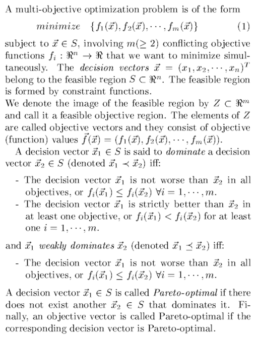
Multi-objective optimization
Since the final goal of this series is the implementation of MOPSO, let us start with the mathematical concept behind multi-objective optimization as reminded in Mostaghim et al. paper [1]:
Our multi-objective problem
We want to use a multi-objective PSO approach to find VaR-efficient portfolios by solving the following optimization problem: [2]
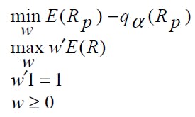
where

Thus, we want to find a set of optimal solutions (weights w') to
minimize de Value-at-Risk (VaR), relative to the mean, of the portfolio
maximize the expected return of the portfolio
Our objective functions
We will define f1 as being the Value-at-Risk (VaR), relative to the mean, of the portfolio, and f2 as the expected return of the portfolio.
Finally, based on the mathematical explanation provided above we want to find the Pareto-optimal decision vectors (or weights) and their corresponding Pareto-optimal objective vector values (black squares in the figure below).
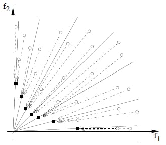
These Pareto-optimal decision vectors (or weights) are also called non-dominated solutions. In a MOPSO context they are also called archive-members.
Packages
Load the following packages:
library(PerformanceAnalytics)
library(quantmod)
library(tidyquant)
library(tidyverse)
library(timetk)
library(skimr)
library(plotly)
library(caret)
library(tictoc)
Collect prices, compute daily returns and clean data
This is the same code used in the Nonparametric VaR article.
# ASSETS
assets <- c("MSFT", "AAPL", "GOOG", "NFLX")

# TIME INTERVAL

end <- "2021-12-31" %>% ymd()
start <- end - years(5) + days(1)

# GET ASSETS' DAILY RETURNS

returns_daily_tbl <- assests %>%
  tq_get(from = start, to = end) %>%
  group_by(symbol) %>%
  tq_transmute(select = adjusted,
               mutate_fun = periodReturn,
               period = "daily") %>%
  ungroup()

# PREPROCESSING - CLEAN

## Delete each asset first row (= 0)
rows_to_delete <- which(returns_daily_tbl$date == ymd("2017-01-03"))
returns_daily_tbl <- returns_daily_tbl[-rows_to_delete,]
Daily returns tibble format
Let us put the tibble in the right format by renaming the columns and converting the symbol column to factor, here below the corresponding custom function:
formatTibble <- function(tbl){
  columnNames <- c("symbol", "date", "returns")
  res <- tbl %>%
    mutate(symbol = as.factor(symbol))
  colnames(res) <- columnNames

  return(res)
}
Get weighted returns
The next custom function getWeigthedReturns() multiplies a weight from the weight vector to its corresponding asset daily returns and outputs an updated tibble with new columns: weight and weighted.returns.
getWeigthedReturns <- function(tbl, vecA, vecW){
  # Generate by-symbol tibble with weighted returns
  # add by-symbol tibble to a list
  lsymboltbl <- lapply(X = 1:length(vecA), function(x){
    tbl %>%
      filter(symbol == vecA[x]) %>%
      mutate(weight = vecW[x]) %>%
      mutate(weighted.returns = returns * weight)
  })

  # Bind symbol tibble by rows
  res <- lsymboltbl %>%
    bind_rows()

  return(res)
}
Compute mean of weighted returns
Our goal here is to generate the same tibble (portfolio) from which we calculated the expected return and the "relative to the mean" VaR in the Nonparametric VaR article. Thus, we group by date and calculate the mean of daily returns of the 4 assets.
getMeanWeigthedReturns <- function(tbl){
  res <- tbl %>%
    group_by(date) %>%
    summarise(mean.weighted.returns = mean(weighted.returns))

  return(res)
}
Objective function f1: VaR
Although the custom function calculates both absolute and relative VaR, we consider only the "relative to the mean" VaR as the output of objective function f1.
objectiveFunction1 <- function(tbl, p = .99){
  # Absolute VaR
  absoluteVaR <- tbl %>%
    tq_performance(Ra = mean.weighted.returns,
                   performance_fun = VaR,
                   p = p,
                   method = "historical")

# Relative VaR: E(Rp) - q(Rp)
  relativeVaR <- mean(tbl$mean.weighted.returns) - absoluteVaR$VaR

  return(list(VaR = list(abolute = absoluteVaR$VaR,
                         relative = relativeVaR)))
}
Objective function f2: Expected return
Since we apply a minimization for both objective functions, the objectiveFunction2() custom function outputs a negative value for the expected return.
objectiveFunction2 <- function(tbl){
  # w'E(R)
  res <- mean(tbl$mean.weighted.returns)
  return(-res)
}
Other custom functions
We will generate 1000 random 4-weight solutions with the generateRandomWeightsVector() custom function. All four weights must sum to 1. I have also added a constraint to avoid generating 0-valued and 1-valued weights.
generateRandomWeightsVector <- function(n, min=.05, max=.75){

  tmp <- runif(n = n, min = min, max = max)
  nweights <- tmp/sum(tmp)

  new_cols <- list()
  for(x in 1:n) {
    new_cols[[paste0("w_", x, sep="")]] = nweights[x]
  }

  res <- as_tibble(new_cols)

  return(res)
}
We group the random solutions with their respective objective functions results in the same tibble with the following custom function:
getObjectiveFunctionsValues <- function(tbl, vecW){

  new_cols <- list()
  for(x in 1:length(vecW)) {
    new_cols[[paste0("w_", x, sep="")]] = vecW[x]
  }
  res <- as_tibble(new_cols)

  objf1val <- objectiveFunction1(tbl)
  objf2val <- objectiveFunction2(tbl)

  res <- res %>%
    mutate(absVaR = objf1val$VaR$abolute) %>%
    mutate(relVaR = objf1val$VaR$relative) %>%
    mutate(expRet = objf2val) %>%
    mutate(pAbsVaR = absVaR * 100) %>%
    mutate(pRelVaR = relVaR * 100) %>%
    mutate(pExpRet = expRet * 100)

  return(res)
}
The tibble generated by the function above will be used to find the non-dominated solutions using the following custom function:
getNonDominated <- function(tbl) {

  idxVar <- which(colnames(tbl) == "relVaR")
  idxExpR <- which(colnames(tbl) == "expRet")

  i <- order(tbl[, idxVar], tbl[, idxExpR], decreasing=FALSE)
  frontier <- rep(0, length(i))
  k <- 0;
  y <- Inf
  for (j in i) {
    if (tbl[j, idxExpR] < y) {
      frontier[k <- k+1] <- j
      y <- tbl[j, idxExpR]
    }
  }
  return(frontier[1:k])
}
Main R code
The code within the tictoc ran for 2 minutes, I have a Windows laptop, i5 CPU (8 vCores), 16GB RAM.
## 1. Create random particles tibble ----

NUMBER_OF_ASSETS = 4
NUMBER_PARTICLES = 1000

lrandomparticles <- lapply(X = 1:NUMBER_PARTICLES, function(x){
  generateRandomWeightsVector(n = NUMBER_OF_ASSETS)
})
random_particles <- lrandomparticles %>%
  bind_rows()

# 1000 random solutions
> random_particles
# A tibble: 1,000 x 4
      w_1    w_2    w_3    w_4
    <dbl>  <dbl>  <dbl>  <dbl>
 1 0.424  0.431  0.0569 0.0873
 2 0.283  0.363  0.126  0.227
 3 0.351  0.258  0.0496 0.341
 4 0.266  0.218  0.431  0.0854
 5 0.225  0.304  0.329  0.142
 6 0.298  0.0952 0.409  0.198
 7 0.190  0.197  0.424  0.189
 8 0.335  0.310  0.264  0.0912
 9 0.0437 0.430  0.274  0.252
10 0.0981 0.413  0.0400 0.449
# ... with 990 more rows

## 2. Generate particle & objective functions' results tibble ----

tic()
lparticlesObjFunResults <- lapply(1:NUMBER_PARTICLES, function(x){

  weights <- as.numeric(random_particles[x,])

  returns_daily_tbl %>%
    formatTibble() %>%
    getWeigthedReturns(vecA = assests, vecW = weights) %>%
    getMeanWeigthedReturns() %>%
    getObjectiveFunctionsValues(vecW = weights) %>%
    mutate(sharpe = expRet/relVaR)

})
toc()

particlesObjFunResults <- lparticlesObjFunResults %>%
  bind_rows()

> particlesObjFunResults
# A tibble: 1,000 x 11
      w_1    w_2    w_3    w_4  absVaR relVaR    expRet pAbsVaR pRelVaR pExpRet sharpe
    <dbl>  <dbl>  <dbl>  <dbl>   <dbl>  <dbl>     <dbl>   <dbl>   <dbl>   <dbl>  <dbl>
 1 0.424  0.431  0.0569 0.0873 -0.0109 0.0113 -0.000396   -1.09    1.13 -0.0396 0.0352
 2 0.283  0.363  0.126  0.227  -0.0106 0.0110 -0.000387   -1.06    1.10 -0.0387 0.0352
 3 0.351  0.258  0.0496 0.341  -0.0107 0.0111 -0.000390   -1.07    1.11 -0.0390 0.0353
 4 0.266  0.218  0.431  0.0854 -0.0110 0.0113 -0.000355   -1.10    1.13 -0.0355 0.0314
 5 0.225  0.304  0.329  0.142  -0.0108 0.0112 -0.000367   -1.08    1.12 -0.0367 0.0329
 6 0.298  0.0952 0.409  0.198  -0.0106 0.0109 -0.000353   -1.06    1.09 -0.0353 0.0324
 7 0.190  0.197  0.424  0.189  -0.0108 0.0111 -0.000355   -1.08    1.11 -0.0355 0.0319
 8 0.335  0.310  0.264  0.0912 -0.0108 0.0111 -0.000373   -1.08    1.11 -0.0373 0.0336
 9 0.0437 0.430  0.274  0.252  -0.0107 0.0110 -0.000376   -1.07    1.10 -0.0376 0.0340
10 0.0981 0.413  0.0400 0.449  -0.0112 0.0116 -0.000396   -1.12    1.16 -0.0396 0.0340
# ... with 990 more rows

ndidx <- getNonDominated(tbl = particlesObjFunResults)

gp <- ggplot() +
  geom_point(particlesObjFunResults[ndidx,], mapping = aes(x = pRelVaR, y = pExpRet), color = "red") +
  geom_point(particlesObjFunResults[-ndidx,], mapping = aes(x = pRelVaR, y = pExpRet), color = "black")
ggplotly(gp)
Be reminded that the objective function f2 outputs negative values for the portfolio expected returns (because we consider a minimization problem, see the figure of Pareto-optimal objective vector at the beginning of the article). Thus, we are actually displaying the frontier upsides down.
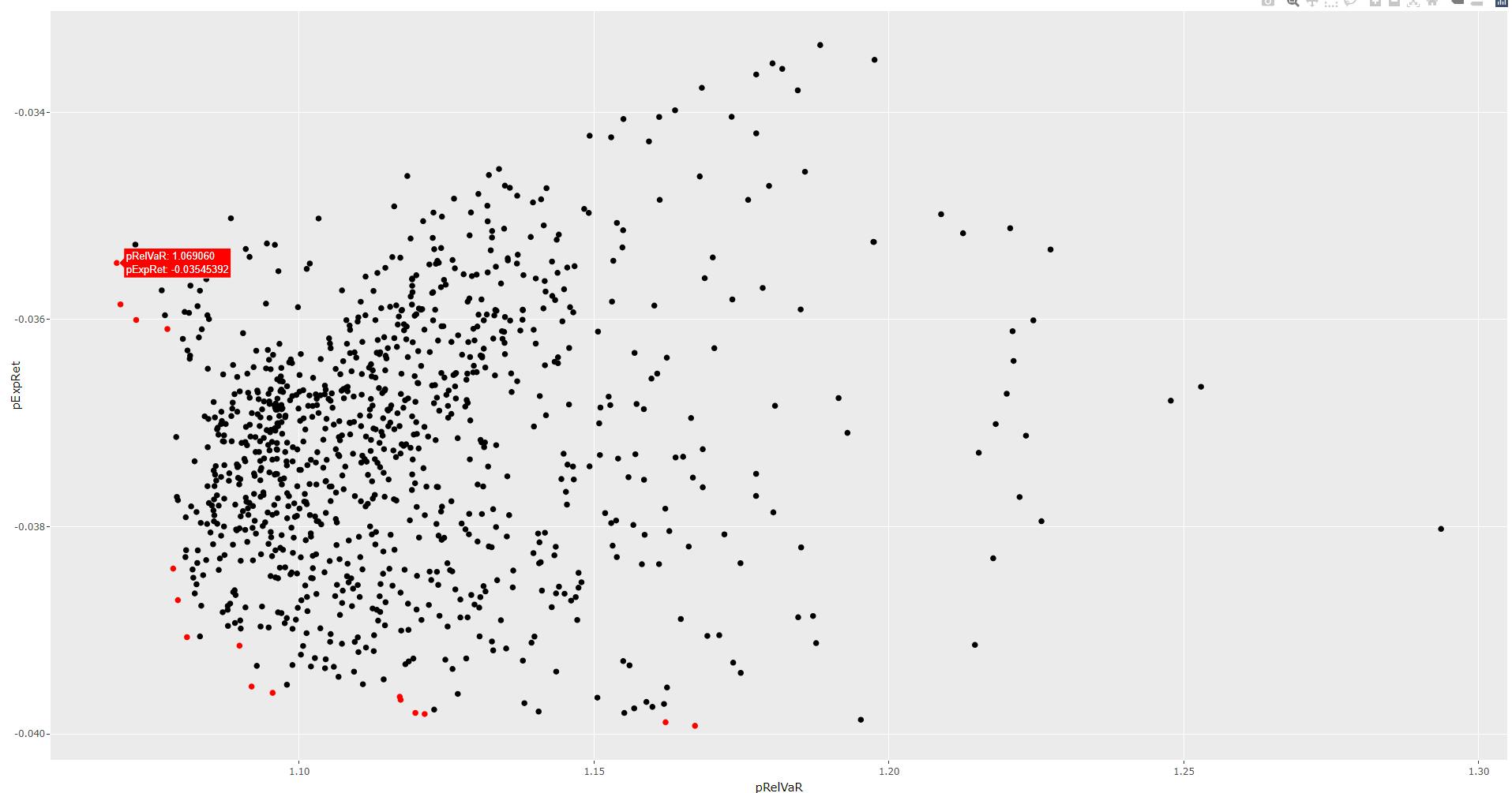
Below you will find the 16 non-dominated solutions (red points) along with their corresponding VaR (%) and expected return (%) results (expressed in percentage), keeping the negative sign of the expected return (%).
In the Nonparametric VaR article we considered an equally distributed weight set (25% weight for each asset) and obtained an expected return of 0.032% and a relative VaR of 1.08%. We see that the first 3 non-dominated solutions below provide a higher expected return (ignore the negative sign) with less risk.
> particlesObjFunResults[ndidx,] %>%
    select(w_1, w_2, w_3, w_4, pRelVaR, pExpRet) %>%
    arrange(pRelVaR)
# A tibble: 16 x 6
     w_1    w_2    w_3   w_4 pRelVaR pExpRet
   <dbl>  <dbl>  <dbl> <dbl>   <dbl>   <dbl>
 1 0.313 0.0748 0.386  0.226    1.07 -0.0355
 2 0.310 0.110  0.354  0.225    1.07 -0.0359
 3 0.283 0.138  0.347  0.232    1.07 -0.0360
 4 0.345 0.0844 0.318  0.252    1.08 -0.0361
 5 0.447 0.193  0.101  0.259    1.08 -0.0384
 6 0.359 0.256  0.0869 0.298    1.08 -0.0387
 7 0.420 0.338  0.0818 0.161    1.08 -0.0391
 8 0.458 0.310  0.0629 0.169    1.09 -0.0391
 9 0.378 0.394  0.0476 0.181    1.09 -0.0395
10 0.302 0.419  0.0466 0.233    1.10 -0.0396
11 0.244 0.481  0.0645 0.211    1.12 -0.0396
12 0.168 0.527  0.0759 0.230    1.12 -0.0397
13 0.217 0.446  0.0313 0.305    1.12 -0.0398
14 0.378 0.453  0.0408 0.128    1.12 -0.0398
15 0.175 0.600  0.0810 0.144    1.16 -0.0399
16 0.105 0.604  0.0752 0.216    1.17 -0.0399
Conclusion
In this article I wanted to illustrate the notion of non-dominated solutions applied to a portofolio optimization use case. Here we started by generating a random set of 1000 weight vectors in order to find the non-dominated solutions among this set of 1000 weight vectors. Our utimate goal will be to generate these weight vectors and non-dominated solutions with the MOPSO algorithm, but first we will explain other notions such as finding good local guides with the Sigma method [1].
References
[1] Mostaghim S., Teich J., « Strategies for Finding Local Guides in Multi-objective Particle Swarm Optimization (MOPSO) »
[2] Alfaro Cid E. et al., « Minimizing value-at-risk in a portfolio optimization problem using a multiobjective genetic algorithm », International Journal of Risk Assessment and Management, 2011