


Part 1 - Nonparametric Value-at-Risk (VaR)
Computing and visualizing nonparametric VaR with R


Cover photo by Chris Liverani on Unsplash
Go to R-bloggers for R news and tutorials contributed by hundreds of R bloggers.
Introduction
This is the first of a series of articles explaining how to apply multi-objective particle swarm optimization* (MOPSO) to portfolio management.
Notion of Value-at-Risk (VaR)
As per P. Jorion's book [1], "we can formally define the value at risk (VaR) of a portfolio as the worst loss over a target horizon such that there is a low, prespecified probability that the actual loss will be larger."
This definition involves two quantitative factors, the horizon and the confidence level.
Define c as the confidence level and L as the loss, measured as a positive number. VAR is also reported as a positive number.
A general definition of VAR is that it is the smallest loss, in absolute value, such that
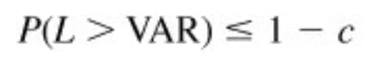
Take, for instance, a 99 percent confidence level, or c = 0.99. VAR then is the cutoff loss such that the probability of experiencing a greater loss is less than 1 percent.
Computing VaR
The figure below comes from a Bionic Turtle video available in YouTube [2], it takes only 6 minutes, have a look!
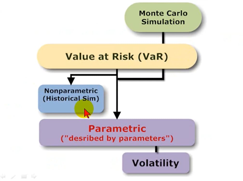
The nonparametric approach uses actual historical data, it is simple and easy to use. There is no hypothesis about the distribution of the data. This is the approach used in this article.
The Monte Carlo simulation is about imagining hypothetical future data. It generates its own data i.e., given a model specification about the assets of the portfolio we run any number of trials in order to obtain a simulated distribution of data.
The parametric approach uses the data (as an excuse) to find a distribution, usually a normal distribution which requires only two parameters: the mean and the standard deviation.
As per [3], "approaches to quantify VaR such as delta-normal, delta-gamma or Monte Carlo simulation method rely on the normality assumption or other prespecified distributions. These approaches have several drawbacks, such as the estimation of parameters and whether the distribution fit properly the data in the tail or not."
Computing nonparametric VaR with R
Example
Below is the example taken from Jorion's book [1]. I'm going to copie his explanation about the VaR computation, and then I will base my explanations and code on my interpretation of Jorion's book [1] explanations and figure.
Assume that this (the nonparametric VaR) can be used to define a forward-looking distribution, making the hypothesis that daily revenues are identically and independently distributed.
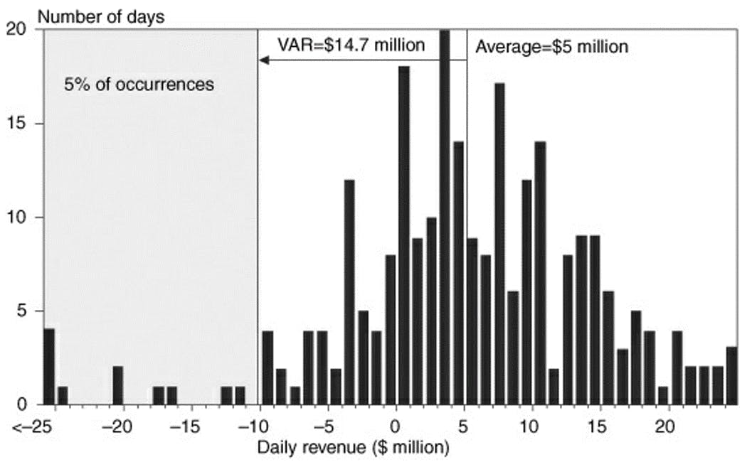
We can derive the VAR at the 95 percent confidence level from the 5 percent left-side “losing tail” in the histogram.
The figure (above), for instance, reports J.P. Morgan’s distribution of daily revenues in 1994. The graph shows how to compute nonparametric VAR.
Let W' be the lowest portfolio value at the given confidence level c.
From this graph, the average revenue is about $5.1 million. There is a total of 254 observations; therefore, we would like to find W' such that the number of observations to its left is 254 × 5 percent = 12.7.
We have 11 observations to the left of −$10 million and 15 to the left of −$9 million. Interpolating, we find W' = −$9.6 million.
The VaR of daily revenues, measured relative to the mean, is VAR = E (W) − W' = $5.1 − (−$9.6) = $14.7 million.
If one wishes to measure VaR in terms of absolute dollar loss, VaR then is $9.6 million.
Finally, it is useful to describe the average of losses beyond VaR, which is $20 million here. Adding the mean, we find an expected tail loss (ETL) of $25 million.*
Basis of my explanation
Let us consider that the daily returns ofthe figure correspond to a portfolio composed of four assets: Microsoft ("MSFT"), Apple ("AAPL"), Google ("GOOG"), and Netflix ("NFLX").
In order to display the histogram we should have a (final) tibble like this one:
# A tibble: 1,257 x 2
   date       mean.weighted.returns
   <date>                     <dbl>
 1 2017-01-04              0.000652
 2 2017-01-05              0.00204
 3 2017-01-06              0.00184
 4 2017-01-09              0.000355
 5 2017-01-10             -0.000607
 6 2017-01-11              0.00144
 7 2017-01-12             -0.00159
 8 2017-01-13              0.00228
 9 2017-01-17             -0.000297
10 2017-01-18              0.000252
# ... with 1,247 more rows
The tibble above has a column called "mean.weighted.returns" which means that we have taken the weighted mean of the assets' daily returns. Here, the weights have been equally distributed e.g., 25% MSFT, 25% AAPL, 25% GOOG, and 25% NFLX.
OK, let us then generate this tibble.
R packages
library(PerformanceAnalytics)
library(quantmod)
library(tidyquant)
library(tidyverse)
library(timetk)
library(skimr)
library(plotly)
Get the data
Let us collect 5 years of data e.g., the prices of the four assets: Microsoft ("MSFT"), Apple ("AAPL"), Google ("GOOG"), and Netflix ("NFLX"). For this, we will use the tq_get() from tidyquant package.
I prefer to use the tidyquant package because I like to work with tibbles, I don't have to worry about the different time series data format (xts, ...).
We will directly compute the daily returns of the adjusted prices.
assests <- c("MSFT", "AAPL", "GOOG", "NFLX")

end <- "2021-12-31" %>% ymd()
start <- end - years(5) + days(1)

returns_daily_tbl <- assests %>%
  tq_get(from = start, to = end) %>%
  group_by(symbol) %>%
  tq_transmute(select = adjusted,
               mutate_fun = periodReturn,
               period = "daily") %>%
  ungroup()

> returns_daily_tbl
# A tibble: 5,032 x 3
   symbol date       daily.returns
   <chr>  <date>             <dbl>
 1 MSFT   2017-01-03      0
 2 MSFT   2017-01-04     -0.00447
 3 MSFT   2017-01-05      0
 4 MSFT   2017-01-06      0.00867
 5 MSFT   2017-01-09     -0.00318
 6 MSFT   2017-01-10     -0.000319
 7 MSFT   2017-01-11      0.00910
 8 MSFT   2017-01-12     -0.00918
 9 MSFT   2017-01-13      0.00144
10 MSFT   2017-01-17     -0.00271
# ... with 5,022 more rows
Clean the data
Because of the daily return calculation, the first row ("2017-01-03") of each asset will be zero. Let us delete these four rows, one per asset (or symbol).
rows_to_delete <- which(returns_daily_tbl$date == ymd("2017-01-03"))
returns_daily_tbl <- returns_daily_tbl[-rows_to_delete,]
Define the weights vector
wts_tbl <- returns_daily_tbl %>%
  distinct(symbol) %>%
  mutate(weight = c(.25, .25, .25, .25))
Apply the weights
Let us apply the weights by creating two new columns, weight and weighted.returns. The symbol column will be converted from character to factor.
returns_daily_weighted_tbl <- returns_daily_tbl %>%
  group_by(symbol) %>%
  mutate(weight = case_when(symbol == "MSFT" ~ as.numeric(wts_tbl[1,2]),
                            symbol == "AAPL" ~ as.numeric(wts_tbl[2,2]),
                            symbol == "GOOG" ~ as.numeric(wts_tbl[3,2]),
                            symbol == "NFLX" ~ as.numeric(wts_tbl[4,2]))) %>%
  mutate(weighted.returns = daily.returns * weight) %>%
  mutate(symbol = as.factor(symbol))

> returns_daily_weighted_tbl
# A tibble: 5,028 x 5
# Groups:   symbol [4]
   symbol date       daily.returns weight weighted.returns
   <fct>  <date>             <dbl>  <dbl>            <dbl>
 1 MSFT   2017-01-04     -0.00447    0.25       -0.00112
 2 MSFT   2017-01-05      0          0.25        0
 3 MSFT   2017-01-06      0.00867    0.25        0.00217
 4 MSFT   2017-01-09     -0.00318    0.25       -0.000796
 5 MSFT   2017-01-10     -0.000319   0.25       -0.0000798
 6 MSFT   2017-01-11      0.00910    0.25        0.00228
 7 MSFT   2017-01-12     -0.00918    0.25       -0.00229
 8 MSFT   2017-01-13      0.00144    0.25        0.000359
 9 MSFT   2017-01-17     -0.00271    0.25       -0.000678
10 MSFT   2017-01-18     -0.000480   0.25       -0.000120
# ... with 5,018 more rows
Compute the mean
Group by date and take the mean of the 4 assets' weighted daily returns.
returns_daily_weighted_mean_tbl <- returns_daily_weighted_tbl %>%
  group_by(date) %>%
  summarise(mean.weighted.returns = mean(weighted.returns))

> returns_daily_weighted_mean_tbl
# A tibble: 1,257 x 2
   date       mean.weighted.returns
   <date>                     <dbl>
 1 2017-01-04              0.000652
 2 2017-01-05              0.00204
 3 2017-01-06              0.00184
 4 2017-01-09              0.000355
 5 2017-01-10             -0.000607
 6 2017-01-11              0.00144
 7 2017-01-12             -0.00159
 8 2017-01-13              0.00228
 9 2017-01-17             -0.000297
10 2017-01-18              0.000252
# ... with 1,247 more rows
And that's it! we have finally obtained the tibble from which we will generate the histogram and calculate the VaR.
Display summary statistics
Let us define a skimr custom function to add the min and max values to the default summary statistics display of the previous tibble.
myskim <- skim_with(numeric = sfl(max, min),
                    append = TRUE)

returns_daily_weighted_mean_tbl %>%
  myskim()

> returns_daily_weighted_mean_tbl %>%
     myskim()
-- Data Summary ------------------------
                           Values
Name                       Piped data
Number of rows             1257
Number of columns          2
_______________________
Column type frequency:
  Date                     1
  numeric                  1
________________________
Group variables            None

-- Variable type: Date ------------------------------------------------------------------------------------------------------------------------------------------
# A tibble: 1 x 7
  skim_variable n_missing complete_rate min        max        median     n_unique
* <chr>             <int>         <dbl> <date>     <date>     <date>        <int>
1 date                  0             1 2017-01-04 2021-12-30 2019-07-05     1257

-- Variable type: numeric ---------------------------------------------------------------------------------------------------------------------------------------
# A tibble: 1 x 13
  skim_variable         n_missing complete_rate     mean      sd      p0      p25      p50     p75   p100 hist     max     min
* <chr>                     <int>         <dbl>    <dbl>   <dbl>   <dbl>    <dbl>    <dbl>   <dbl>  <dbl> <chr>  <dbl>   <dbl>
1 mean.weighted.returns         0             1 0.000372 0.00407 -0.0312 -0.00131 0.000547 0.00230 0.0264 ▁▁▇▂▁ 0.0264 -0.0312
From the skimr resut above we can see that the mean of mean.weighted.returns (or the portfolio Expected Return) is 0.000372 or 0.037%. You can also have a quick look at the displayed (mini) histogram provided.
Compute nonparametric VaR
To compute the absolute nonparametric VaR at 99% confidence level with use the tidyquant::tq_performance() function. Thus, you must specify:
Ra: the column of asset returs (here, the mean.weighted.returns)performance_fun: the performnace function (here, the VaR)p: here, the confidence level (99%)method: for nonparametric VaR we use the historical method as explained at the beginning of the article.
VaR.tq <- returns_daily_weighted_mean_tbl %>%
tq_performance(Ra = mean.weighted.returns,
performance_fun = VaR,
p = .99,
method = "historical")
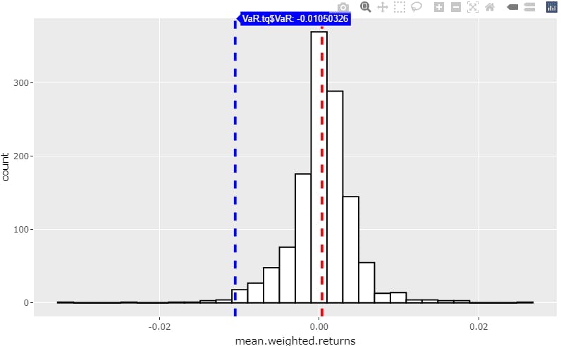
> cat("VaR @99% = ", VaR.tq$VaR)
VaR @99% = -0.01050326
We obtain the absolute VaR @99% = -0.01050326, this is the cutoff loss such that the probability of experiencing a greater loss is less than 1 percent.
The relative (to the mean) VaR @99% should be 0.000372 - (-0.01050326) = 0.01087526, let us check:
> mean(returns_daily_weighted_mean_tbl$mean.weighted.returns) - VaR.tq$VaR
[1] 0.0108755
Here, for this fictitious example, we consider the holding period = 1 day. Since we are computing a nonparametric VaR for which no hypothesis of the distribution e.g., normality, has been made, we cannot apply the "VaR(T days) = VaR*SQRT(T)" rule.
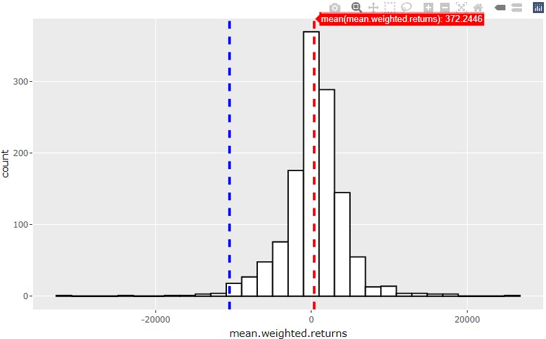
Visualize nonparametric VaR
gp <- ggplot(returns_daily_weighted_mean_tbl, aes(x=mean.weighted.returns)) +
  geom_histogram(color="black", fill="white") +
  geom_vline(aes(xintercept=VaR.tq$VaR), color="blue", linetype="dashed", size=1)
ggplotly(gp)
Apply positions amount
Let us consider an investment of $1,000,000 which has been equally distributed across all four assets e.g., 25% per asset thus, $250,000 per asset.
The portfolio Expected Return is 0.000372 of $1,000,000 = $372
The absolute VaR @99% is -0.01050326 x $1,000,000 = -$10,503.26, this is the cutoff loss such that the probability of experiencing a greater loss is less than 1 percent.
The relative (to the mean) VaR @99% is $372 - (-$10,503.26) = $10,875.26
Change the weights
Say we apply the following weights to the four assets:
> wts_tbl2
# A tibble: 4 x 2
  symbol weight
  <chr>   <dbl>
1 MSFT     0.2
2 AAPL     0.15
3 GOOG     0.15
4 NFLX     0.5
The portfolio Expected Return is $377
The absolute VaR @99% is -$11,228, this is the cutoff loss such that the probability of experiencing a greater loss is less than 1 percent.
The relative (to the mean) VaR @99% is $11,606
Consequently, by applying these new weights we have increased the VaR of the portfolio. Thus, in terms of risk management, this new set of weights was not a good choice.
Towards portfolio optimization
Now, in terms portfolio optimization when considering the following objective function which is the minimization of the VaR relative to the mean equation:
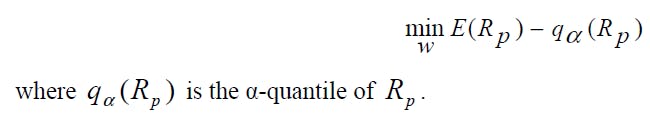
the investor preferences are expressed as a function of return and maximum loss, and a VaR-efficient frontier (made up of Pareto efficient portfolios) in the mean-VaR space has to be found. For this reason, we will use multiobjective PSO approach to find VaR-efficient portfolios by solving the following optimization problem: [3]
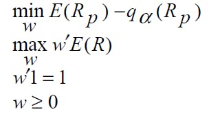
This is the goal of this series of articles covering the application of MOPSO algorithm to portfolio optimization.
References
[1] Jorion, Philippe "Value-at-Risk", Third Edition
[2] FRM: Three approaches to value at risk (VaR), Bionic Turtle, 16 juil. 2008, YouTube.
[3] Alfaro Cid E. et al., « Minimizing value-at-risk in a portfolio optimization problem using a multiobjective genetic algorithm », International Journal of Risk Assessment and Management, 2011